Convolutional Neural Networks (CNNs): Concept And Application
In the previous tutorial on Introduction to Artificial Neural Networks (ANNs), we explored the fundamentals of deep learning and witnessed the capabilities of fully connected neural networks in tackling various tasks. We delved into how neurons within FNNs connect to solve basic problems like regression and classification. However, the human brain excels at solving significantly more intricate tasks beyond the capabilities of FNNs. To address these challenges, we have developed various types of artificial neurons, each tailored for specific problems. For instance, image and video processing requires a more complex architecture than traditional FNNs can offer. This is where convolutional neural networks (CNNs) come into play, offering a powerful tool to tackle these intricate data types.
Table of Contents
Prerequisites:
- Python, Numpy, Sklearn, Pandas and Matplotlib.
- Familiarity with TensorFlow and Keras
- Linear Algebra For Machine Learning.
- Statistics And Probability Theory.
- All of our previous machine-learning tutorials
-
Sale Product on sale
 Linear Algebra For Machine Learning And Data Science
40.00$Original price was: 40.00$.24.99$Current price is: 24.99$. -
Sale Product on sale
 Probability and Statistics for Machine Learning and Data Science
30.00$Original price was: 30.00$.19.00$Current price is: 19.00$.
Why Convolutional Neural Networks And Not FNN?
Imagine using a fully connected neural network (FCN or FNN) for image recognition. The first major hurdle is the sheer number of neurons needed in the first layer, as even a small image has thousands of pixels, each requiring a corresponding neuron in the FNN. These neurons would then be fully connected to each other, creating an intricate network of connections. However, this complexity comes at a cost. The network wouldn’t inherently understand the crucial higher-dimensional arrangement of pixels in an image, making it difficult to learn meaningful features. Furthermore, training such a network with huge parameters or with its massive number of connections becomes a computationally challenging task.
However, it’s important to note that while FCNs can learn some spatial information, they struggle significantly compared to approaches specifically designed to handle the 2D (when width and height) or 3D ( when we also take depth into account) structure of images (CNNs in our case). Spatial information here means the relative arrangement and positions of pixels within an image. Spatial information can allow us to understand the outline, shapes, depth and even recognize patterns within an image. This is why we don’t use FNNs or FCNs for image recognition tasks.
A fully connected first layer with, say, one hundred hidden units would already contain several tens of thousands of weights. Such a large number of parameters increases the capacity of the system and therefore requires a larger training set. In addition, the memory requirement to store so many weights may rule out certain hardware implementations. But the main deficiency of unstructured nets for image or speech applications is that they have no built-in invariance with respect to translations or local distortions of the inputs.
Before being sent to the fixed-size input layer of a neural net, character images or other 2D or 3D signals must be approximately size-normalized and centered in the input field. Unfortunately, no such preprocessing can be perfect; handwriting is often normalized at the word level, which can cause size, slant, and position variations for individual characters. This, combined with variability in writing style, will cause variations in the position of distinctive features in input objects.
In principle, a fully connected network of sufficient size could learn to produce outputs that are invariant with respect to such variations. However, learning such a task would probably result in multiple units with similar weight patterns positioned at various locations in the input to detect distinctive features wherever they appear. Learning these weight configurations requires a very large number of training instances to cover the space of possible variations.
In convolutional networks, described below, shift invariance is automatically obtained by forcing the replication of weight configurations across space.
Secondly, a deficiency of fully connected architectures is that the topology of the input is entirely ignored. The input variables can be presented in any fixed order without affecting the outcome of the training. On the contrary, images (or time-frequency representations of speech) have a strong 2D local structure; variables (or pixels) that are spatially or temporally nearby are highly correlated. Local correlations are the reasons for the well-known advantages of extracting and combining local features before recognizing spatial or temporal objects, because configurations of neighboring variables can be classified into a small number of categories (e.g., edges, corners). Convolutional Networks force the extraction of local features by restricting the receptive fields of hidden units to be local.
GradientBased Learning Applied to Document Recognition
To understand the concept behind CNNs, we need to understand the basics of an image.
What Is An Image?
To understand digital images, you should have a look at the picture below. It shows how we capture an image. There are various steps involved here:
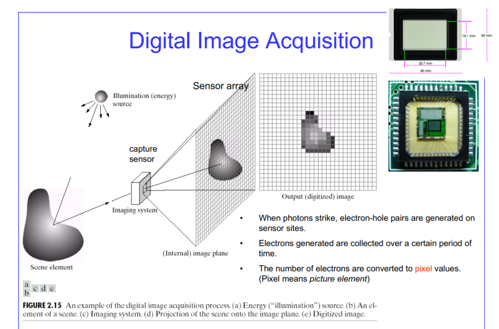
Capturing the Light:
- The Optical System: A camera, whether it’s a traditional film camera, a digital camera, or even your own eye, uses a lens or a system of lenses to focus incoming light onto a sensor.
- The Sensor: The sensor is responsible for converting photons of light into electrical signals. The image sensor is covered with millions of tiny light-sensitive elements called photodetectors. These are like little buckets ready to collect the focused light.
- Light to Electricity: Each photodetector converts the light that falls on it into a proportional electrical signal. The brighter the light, the stronger the signal. This process happens individually for each of the millions of photodetectors.
- Analog Signal: The output from each photodetector is an analogue electrical signal. This means the signal’s value varies continuously based on the intensity of light hitting that specific photodetector.
- The Raw Image: At this stage, we conceptually have a ‘raw’ image. This raw image is a direct representation of the light intensities captured by the sensor, containing all the information needed to create a visible image, but without any post-processing like noise reduction or color correction.
From Electrical Signal to Digital Image:
The analogue electrical signal (which varies continuously based on light intensity) from each photodetector is passed through an analogue-to-digital converter (ADC). The ADC samples this continuous signal at regular intervals and converts each sample into a discrete digital value, representing the light intensity at that specific point.
In this step, we need to understand bit. A bit (short for binary digit) is the smallest unit of information in computing. It has two possible states: 0 or 1. Quantization is the process of converting a continuous range of values (like the intensity of light hitting a photodetector) into a limited set of discrete values. Let’s say our image sensor can only detect two levels: “light” or “dark”. This you can call 1-bit ADC. Let’s say our photodetector receives some light. Think of its analogue signal strength as a scale from 0 (no light) to 1(maximum light). Let’s say the signal strength is 0.8 (bright, but not the maximum). Our 1-bit ADC can’t directly represent 0.8. So, it asks “Is the light above halfway (0.5)?”. Since the answer is yes, it approximates it to the highest level it can represent: 1. The pixel corresponding to that photodetector gets a digital value of 1, representing “light”. Please note: the 1-bit ADC example is an oversimplification for illustrative purposes
Every image is recorded as numerical arrays of pixels. A pixel has its size and bit depth. Bit depth is nothing but what I just explained (intensity). Let’s take another example:
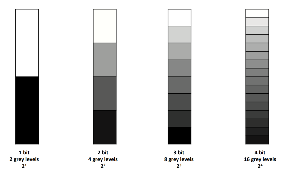
3-bit ADC example: Imagine a single photodetector on our image sensor. Let’s assume: the maximum light intensity for the sensor maps to 5 volts (5V) and no light results in 0 volts. (0V). Our 3-bit ADC divides the 5V range into 8 equally-spaced quantization levels. Each level will be 5V/8 = 0.625V apart.
| Voltage Range | Digital Value (Binary) | Level |
|---|---|---|
| 4.375V to 5V | 111 | 7 |
| 3.75V to 4.375V | 110 | 6 |
| … | … | … |
| 0V to 0.625V | 000 | 0 |
Let’s say the photodetector measures 2.5V of light hitting it. According to the table, this falls into level 4, getting a digital value of 011 (binary) or 3 (decimal). This digital value ‘3’ becomes the intensity value of a single pixel. Each photodetector on the sensor goes through this process and we end up with a matrix of numbers (e.g., 0, 3, 6, 1, 7…) representing the entire image in a discrete format.
Image Representation
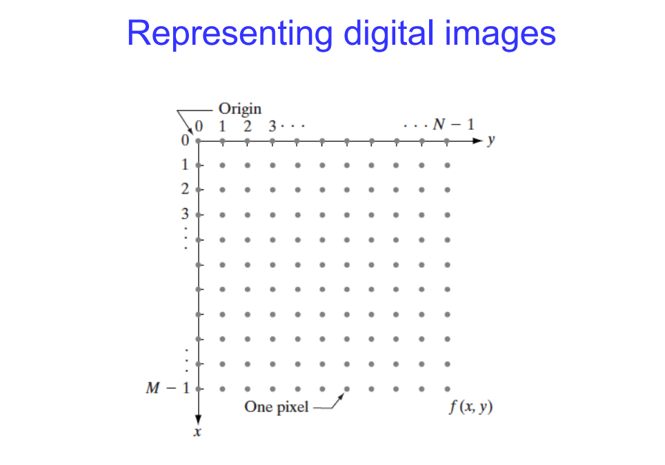
A pixel, short for “picture element,” is the fundamental unit of a digital image. It’s the smallest indivisible unit that contains information about the image’s colour and brightness. Imagine it as a tiny square on a grid overlaying the image. Pixels don’t have an inherent physical size. Their perceived size depends on factors like image resolution (higher resolution images have more pixels crammed into the same physical space, resulting in smaller-looking pixels and creating sharper details), and display size (on a larger display, each pixel occupies a bigger area, making the image appear larger).
Each pixel carries information about its colour or intensity. This information is stored using bits, bit depth as explained earlier refers to the number of bits used to represent the colour or intensity of a single pixel. Higher bit depth signifies more information stored per pixel, leading to a wider range of colours or shades of grey that can be displayed. Higher pixel count and higher bit depth together create a more detailed and realistic image with smoother colour transitions and richer visual depth.
Now, let’s make this whole thing clear using one more example:
Imagine a simple image of a red apple on a green background. Think of the image as a grid of tiny squares, each representing a pixel. Let’s say, for simplicity, our image has a resolution of 4 x 4 pixels. Each pixel doesn’t store colour directly. Instead, it uses channels to represent the colour components. We’ll use the common RGB (Red, Green, Blue) system. So, each pixel has 3 channels, one for each colour. Let’s assume each channel has a bit depth of 3, meaning it can store values from 0 to 7 (2 raised to the power of 3 = 8 possibilities).
| Pixel | Red Channel | Green Channel | Blue Channel |
|---|---|---|---|
| 1,1 | 7 | 0 | 0 |
| 1,2 | 5 | 3 | 0 |
| 1,3 | 2 | 5 | 0 |
| 1,4 | 0 | 7 | 0 |
| 2,1 | 7 | 0 | 0 |
| 2,2 | 0 | 7 | 0 |
| 2,3 | 0 | 7 | 0 |
| 2,4 | 0 | 7 | 0 |
| 3,1 | 2 | 5 | 0 |
| 3,2 | 0 | 7 | 0 |
| 3,3 | 0 | 7 | 0 |
| 3,4 | 0 | 5 | 7 |
| 4,1 | 0 | 7 | 0 |
| 4,2 | 0 | 7 | 0 |
| 4,3 | 0 | 5 | 7 |
| 4,4 | 0 | 0 | 7 |
Images In CNN Input
We usually pass images in a 3D array in its input layer in CNN. This also means you can perform all sorts of mathematical operations. Let me give you an example of how images are represented in CNN:
This is a grayscale image with dimensions 3x3 pixels. Each pixel has a single intensity value:
[ 50, 100, 150 ]
[ 75, 125, 175 ]
[ 25, 200, 255 ]

The image has a height of 3 pixels, a width of 3 pixels, and there's only one color channel (grayscale).
Here:
1. Pixel: Each entry in the 2D array represents a pixel, corresponding to a single intensity value in a grayscale image.
2. Bit Depth: In this case, if using 8 bits per pixel, the bit depth is 8, allowing for 256 possible intensity values.
3. Channels: For grayscale images, there is only one channel, representing the intensity or brightness of each pixel.
Now let's see RGB image. This is how you can represent them in 3-D array.

[  [ (50, 0, 0), (100, 50, 0), (150, 100, 0) ],
  [ (75, 25, 0), (125, 75, 25), (175, 125, 75) ],
  [ (25, 0, 25), (200, 100, 50), (255, 150, 100) ]
]

The same matrix can be plotted this way using their co-ordinates:

[  [[50, 0, 0], (pixel at (0,0))
    [100, 50, 0], (pixel at (0,1))
    [150, 100, 0] (pixel at (0,2))
  ],
  [ [75, 25, 0], (pixel at (1,0))
    [125, 75, 25], (pixel at (1,1))
    [175, 125, 75] (pixel at (1,2))
  ],
  [ [25, 0, 25], (pixel at (2,0))
    [200, 100, 50], (pixel at (2,1))
    [255, 150, 100] (pixel at (2,2))
  ]
]


1. In the RGB image, each pixel is represented as a tuple of three values (R, G, B), where R, G, and B are the intensity values for the Red, Green, and Blue channels, respectively. For example, the pixel at position (0,0) has the RGB values [50, 0, 0].

2. In the given example, each intensity value (in the Red, Green, and Blue channels) is typically represented using 8 bits, allowing for values in the range of 0 to 255. So, the bit depth for each channel in this example is 8 bits.

3. Each channel contains the intensity values for its respective color. For instance, the Red channel contains the intensity values for the red color in each pixel. The example array has three channels, one for each color channel: (R, G, B).
But how does computer stores these images? Each intensity value in the RGB tuple (R, G, B) is represented by 8 bits (1 byte).
The binary representation of these values ranges from 00000000 to 11111111 (0 to 255 in decimal). For example:
(50, 0, 0) => (00110010, 00000000, 00000000)
The Red channel (50) is represented as 00110010 in binary.
The Green channel (0) is represented as 00000000 in binary.
The Blue channel (0) is represented as 00000000 in binary.
This process is repeated for each pixel in the image. The binary representations of the RGB values for all pixels are stored in memory sequentially.Code language: JavaScript (javascript)In CNN, when we pass these images through the convolution layers, we perform calculations on these metrics to determine shapes such as edges, lines, etc., in the image.
I hope the above details gave you an idea of how images are processed. For more details on images, I have mentioned some sources in the footnotes; check them out. The above-mentioned details are not exhaustive, but you don’t need to know everything except for the examples in this section. Additionally, here are some awesome videos that will help you get an idea of what actually happens in images, videos, and cameras. I am sharing them here; watch and then move ahead. Also, for more on resolution and image file size visit this here and here.
What Is Video?
I will talk about videos in more detail when we are working on projects related to video but this is an amazing one you should not skip.
Now that we have some basic understanding of images. Let’s move forward and talk about how CNN models learn to recognize images.
How CNN Based Models Work?
To understand CNN, we need to know what kernels or filters are in CNN. In order to learn to detect some elements in the input image data, we use small detectors called filters or kernels. These detectors identify edges or shapes in the input data and learn new features as we go deeper into the layers. Each filter/kernel is a small 2D (or sometimes 3D for video) grid filled with numbers (weights). The size of the filter depends on the specific CNN architecture. The core function of a filter is to detect specific features within the image data. These features could be edges, corners, shapes, textures, or any other visual pattern relevant to the task at hand.
CNN Basics: Filters/Kernels, Convolution, Padding And Strides
So, how exactly do filters work to identify patterns in the images? During the forward pass of a CNN, a filter slides (convolves) across the entire input image, one pixel at a time. At each location, the filter performs an element-wise multiplication between its weights and the corresponding pixel values within a specific region of the image called the receptive field. This region has the same size as the filter itself. The results of these multiplications are then summed up and often passed through an activation function to create a single output value for that location in the feature map. As the filter slides across the entire image, it generates a new 2D map (called a feature map) that highlights the presence of the features the filter was designed to detect. Strong activation values in the feature map indicate a good match between the filter and the image content.
A CNN typically uses multiple filters within a convolutional layer, each with different weight values. This allows the network to learn and detect a variety of features from the image. For example, one filter might be designed to detect horizontal edges, another might detect vertical lines, and another might be sensitive to specific color combinations. By using a combination of filters, CNN builds a richer understanding of the image content. Filters/kernels are not explicitly created or designed by humans. The initial values for the filter weights are randomly assigned. During the training process of a CNN, these weights are updated iteratively based on the training data and the loss function through backpropagation. As the network trains, the weights in the filters adapt to better detect the features relevant to the specific task the CNN is learning.
As you move deeper into the network, filters often learn to detect more complex and abstract features. For instance, early layers might detect simple edges, and deeper layers might learn to recognize complex shapes or even objects.
Traditionally, filters were designed but in CNN filters are learned. Here I will show you can example of how things work but first, let’s see what is a convulation operation.
Grayscale Image (4x4):
[
  [50, 75, 100, 125],
  [150, 175, 200, 225],
  [100, 125, 150, 175],
  [25, 50, 75, 100]
]


Now let's take a Filter (3x3)
[
  [1, 0, -1],
  [1, 0, -1],
  [1, 0, -1]
]

Now, convolution is a process of multiplying this filter to the image elementwise. Since our image is (4 * 4) and filter is (3 * 3), we will slide this filter over the image to perform convolution operation to get our feature map.  Technically, it is a cross-correlation but in CNN we call it convolution. In actual convolution we flip the filters before sliding. Now let's see how we do that:

Initial Position of the Filter Will be Top-left corner of the image:

Filter:
  [1, 0, -1]
  [1, 0, -1]
  [1, 0, -1]

Image Region:
  [50, 75, 100]
  [150, 175, 200]
  [100, 125, 150]

Element-wise Multiplication and Sum or convolution operation:

Element-wise Multiplication:

  [50*1, 0*0, -100*(-1)] + [75*1, 0*0, -125*(-1)] + [100*1, 0*0, -150*(-1)]
  [150*1, 0*0, -200*(-1)] + [175*1, 0*0, -225*(-1)] + [200*1, 0*0, -175*(-1)]
  [100*1, 0*0, -150*(-1)] + [125*1, 0*0, -175*(-1)] + [150*1, 0*0, -200*(-1)]

Sum of Results: 1025

After that we will slide the filter to the next region:
Filter:
  [1, 0, -1]
  [1, 0, -1]
  [1, 0, -1]

Image Region:
  [75, 100, 125]
  [175, 200, 225]
  [125, 150, 175]

Element-wise Multiplication:
  [75*1, 0*0, -125*(-1)] + [100*1, 0*0, -150*(-1)] + [125*1, 0*0, -175*(-1)]
  [175*1, 0*0, -225*(-1)] + [200*1, 0*0, -250*(-1)] + [225*1, 0*0, -275*(-1)]
  [125*1, 0*0, -175*(-1)] + [150*1, 0*0, -200*(-1)] + [175*1, 0*0, -225*(-1)]

Sum of Results: -1275

We will keep sliding the filter over next region and so on until we have covered the entire image. The feature maps resulted from these operations are stacked together and are then passed through activation function, and then to the next layer for learning higher features.

Stacked Feature Maps:
[  [1025],
  [-1275]
]
You have basically, imagine these images in terms of numbers to visualize them in your mind. In CNN, we use multiple filters, so we have to perform multiple operations in one go:
An RGB image:
[  [(255, 0, 0), (0, 255, 0), (0, 0, 255)],
  [(128, 128, 0), (128, 0, 128), (0, 128, 128)],
  [(255, 255, 255), (0, 0, 0), (128, 128, 128)]
]
Let's consdier some filters. These filters you can say are manually desined. These are automatically learned by the model during training.

1. Edge Detection Filter:

[  [-1, -1, -1],
  [-1,  8, -1],
  [-1, -1, -1]
]

2. Horizontal Line Detection Filter:

[  [1, 1, 1],
  [0, 0, 0],
  [-1, -1, -1]
]

3. Vertical Line Detection Filter:
[
  [1, 0, -1],
  [1, 0, -1],
  [1, 0, -1]
]

We will now perfom convoltion for each filters and the appply relu, afterwards, we will stack the feature maps:

Edge Detection Filter Convolution Result:

[  [-382, -128, -255],
  [-128, 0, -128],
  [-382, -128, -255]
]

Horizontal Line Detection Filter Convolution Result:
[
  [255, 0, -255],
  [255, 0, -255],
  [255, 0, -255]
]

Vertical Line Detection Filter Convolution Result:
[
  [255, 128, -255],
  [255, 0, -255],
  [255, 128, -255]
]


Now, Apply Relu
Edge Detection Filter ReLU Activation Result:
[
  [0, 0, 0],
  [0, 0, 0],
  [0, 0, 0]
]

Horizontal Line Detection Filter ReLU Activation Result:
[
  [255, 0, 0],
  [255, 0, 0],
  [255, 0, 0]
]

Vertical Line Detection Filter ReLU Activation Result:
[
  [255, 128, 0],
  [255, 0, 0],
  [255, 128, 0]
]

Now stack them for the next layer:

Stacked Activation Maps:
[
  [
    [0, 0, 0],
    [0, 0, 0],
    [0, 0, 0]
  ],
  [
    [255, 0, 0],
    [255, 0, 0],
    [255, 0, 0]
  ],
  [
    [255, 128, 0],
    [255, 0, 0],
    [255, 128, 0]
  ]
]

This process continues in deeper layers. During training model learn these filters to better indentify these images.
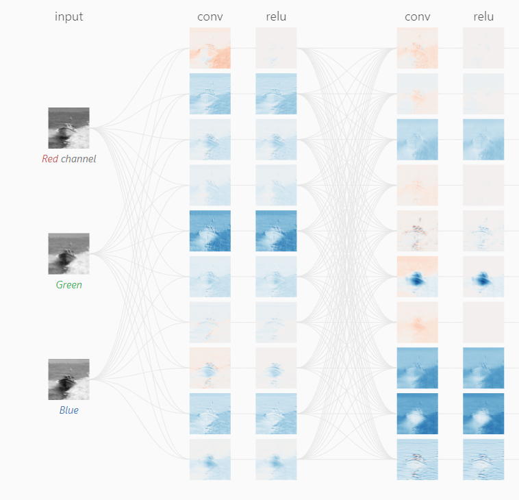
Now one way to visualize this is by using CNN explainer. It’s an interesting way to visualize the filters and all the operations:
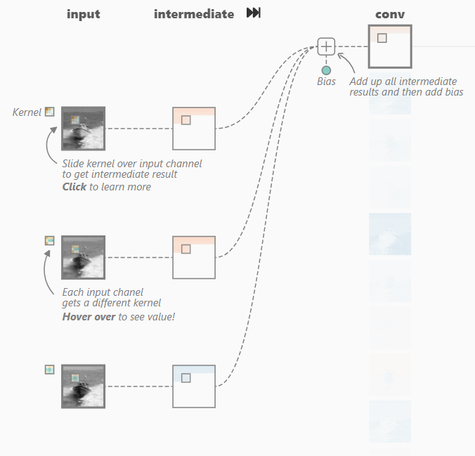
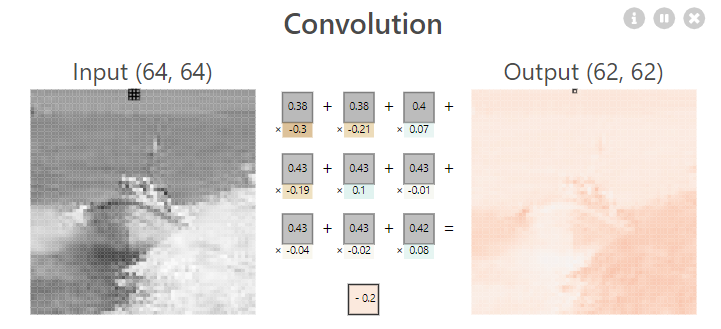
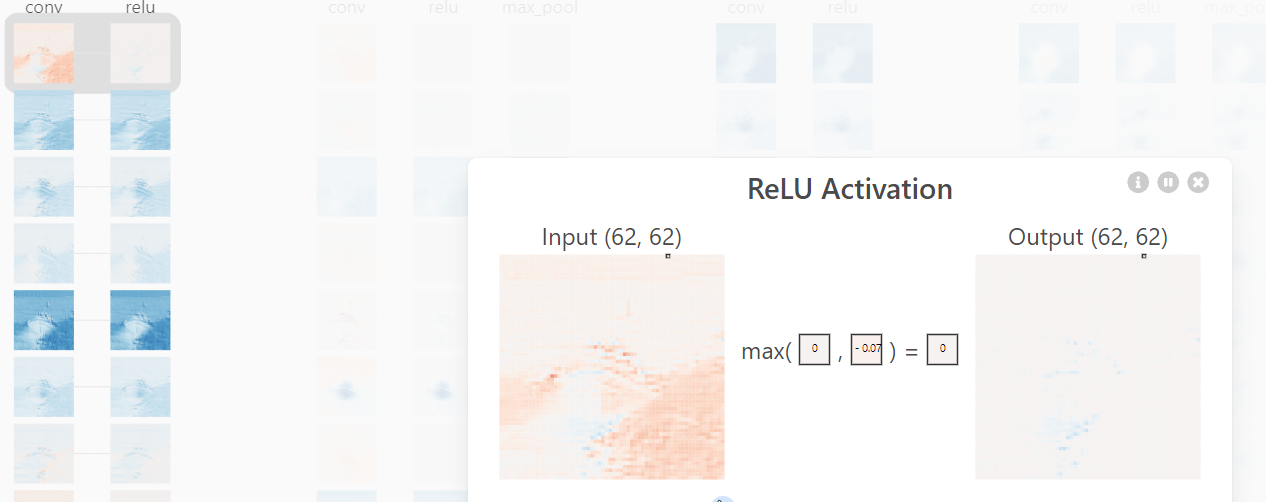
Some key points from the previous explanations that you should keep in mind:
- Convolution helps CNNs extract local features from images.
- The size and weights of the filters or kernels determine what kind of features are detected. Filters can be manually defined for various use cases but in CNN, they are learned during training.
- In RGB images, convolution is applied to each color channel separately, resulting in multiple feature maps.
- Feature maps are combined to create a richer representation of the image for further processing in the CNN.
Each filter in a convolution layer can also have an associated bias term. This is a single value added to the element-wise multiplication and summation during the convolution operation. Mathematically, the convolution operation with bias can be represented as:
Output[i, j] = Σ ( K[p, q, c] * I[i + p, j + q, c] ) + bias_c for all p, q in filter sizeOutput[i, j] is the element at position (i, j) in the feature map.
K[p, q, c] is the weight at position (p, q) in the filter for channel c.
I[i + p, j + q, c] is the pixel value at position (i + p, j + q) in channel c of the input image.
bias_c is the bias term associated with channel c of the filter.Code language: CSS (css)The bias term allows the network to adjust the overall activation of the feature map. This is important because the convolution operation alone might not be sufficient to learn the desired activation level for each element in the feature map. During training, the bias term is adjusted along with the filter weights using backpropagation, allowing the network to learn the optimal bias value for each filter in each channel.
Applying convolutions to images can sometimes affect their size. Padding and strides are two techniques used to control this effect and manipulate the output dimensions of convolutional layers. As we have seen above we are applying filters by shifting them one position at a time, applying filters with a stride of 1 (no skipping pixels) to an image can shrink its width and height after the convolution operation. This is because the filter only overlaps with a portion of the input at each location. The padding adds extra pixels around the border of the input image. This allows the filter to “see” more of the original image and helps maintain the spatial dimensions. Stride is nothing but the step size where as padding is adding some zeros around the border of the image matrix so that we can access all the pixels in it.
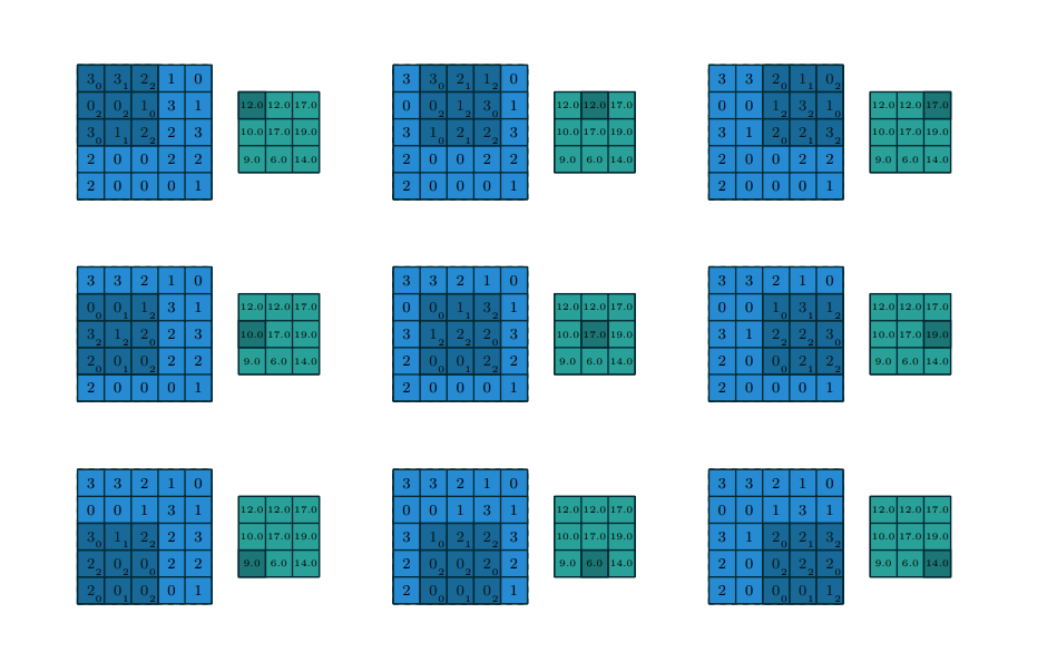
depth of the input feature map.4
Here is an example of padding and strides 2:
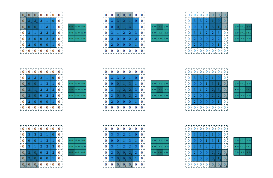
with a 1 × 1 border of zeros using 2 × 2 strides. Notice, how our kernel is moving after skipping 2 steps, and we have also added zero padding to reduce the loss of information. 5
When to Use Strides? When you want to reduce the dimensionality of the data for computational efficiency. This can be helpful in deeper layers of a CNN, and you want to capture higher-level features that are not dependent on the exact location of pixels in the image. For example, a large filter with a stride can detect the presence of an object without needing to pinpoint its exact location.
When to Use Padding? When you want the output feature map to have the same dimensions (width and height) as the input image. This can be important for tasks like image segmentation or dense prediction (predicting a value for each pixel). You want to avoid losing information from the edges of the image, especially for tasks where edge information is important.
Implementation Of the Above Concepts Within The Model Layers In CNN
In a Convolutional Neural Network (CNN), the Convolutional Layer serves as a fundamental building block. It comprises learnable filters, or kernels, typically square matrices with both width and height dimensions. These filters are applied across the width and height of the input volume, extending through its entire depth. The result is a set of 2-dimensional activation maps, each produced by one filter. After applying all K filters to the input volume, these activation maps are stacked along the depth dimension, forming the final output volume.
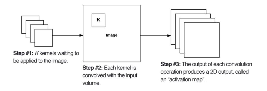
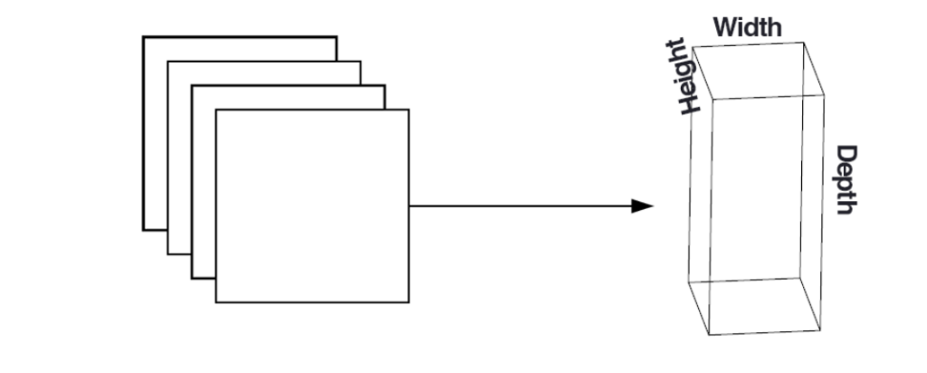
volume to the next layer in the network.7 Several factors influence the size of the output volume (the 3D tensor generated by the CONV layer): Depth (K): The number of filters used in the layer (number of feature maps) Stride (S): The step size between filter applications (S=1 for no skipping, S=2 for skipping one pixel). Smaller strides lead to larger output volumes due to more overlap. Zero-padding (P): Adding zeros around the borders of the input to maintain size or create a specific output size. The formula for calculating the output volume size (assuming square input images):
((W - F + 2P) / S) + 1 W: Width of the input image, F: Size of the filter P: Zero-padding amountEach filter in the CONV layer “looks” at only a small region of the input, reducing the number of connections and parameters needed, and making training more efficient. The size of the receptive field (the area of the input image in the CONV layer considered) is determined by the filter size. Multiple filters contribute to understanding different features in the image, leading to a richer representation of the image data. Neurons in CNN sense you can imagine as convolution operation followed by activation operation but unlike fully connected layers, we only deal with the small region at a time.
Benefits of the Convolutional Layer:
- Feature Extraction: By using multiple filters, the CONV layer extracts a rich set of features from the image, providing a more comprehensive representation for further processing in the network.
- Local Connectivity: Neurons in the CONV layer only connect to a small region of the input, reducing the number of parameters and making the network more efficient to train.
- Shared Weights: Each filter has its own set of learnable weights. Shared weights mean that the same set of filter weights is used across different spatial locations of the input data for each filter. For each filter, the same weights are applied to every receptive field (local region) as the filter slides over the input. By sharing weights, the model reduces the number of parameters to be learned. This parameter sharing is motivated by the assumption that the same feature detector (filter) can be effective in detecting a certain pattern or feature in different parts of the input. Another benefit is translation invariance which means shared weights enable the model to be invariant to translations in the input data. A feature detected in one spatial location can be detected in a different location by the same filter.
Activation Function
After the convolutional operation, which produces the output volume, the activation function is applied to each element (neuron) in the volume individually. Let’s say we have an output volume resulting from a convolutional layer, represented as a 3D array. Each element in this array corresponds to the activation of a neuron in the layer. The activation function is applied element-wise to each neuron’s activation in the output volume. For each element (neuron), the activation function is applied independently.
Suppose we’re using the Rectified Linear Unit (ReLU) activation function, which sets negative values to zero and leaves positive values unchanged. After applying the activation function to each neuron’s activation in the output volume, we get a new volume with transformed activations. The transformed activations now have the non-linear properties introduced by the activation function, enabling the network to learn complex patterns and relationships in the data.
Output (Before Activation) Before Activation:
[
[a, b, c],
[d, e, f],
[g, h, i]
]

Now, the ReLU activation function is applied element-wise to get the new volume:
[
  [max(0, a), max(0, b), max(0, c)],
  [max(0, d), max(0, e), max(0, f)],
  [max(0, g), max(0, h), max(0, i)]
]
Pooling Layers
After this, we often pass the output to the pooling layers. These layers perform a down sampling operation on the activated feature maps, reducing their spatial dimensions (width and height) while retaining important information (similar to increasing sliding window or stride in convolution layer). Pooling shrinks the size of feature maps, leading to fewer parameters in the network. This translates to faster training, lower memory requirements, and reduced risk of overfitting. : Pooling captures the most prominent features within a small region. This makes the network more robust to small shifts or translations in the input, improving generalization to unseen data.
There are two main types of pooling layers:
Max Pooling: This method takes the maximum value from a predefined rectangular region (often a 2×2 window) in the feature map. It essentially identifies the most active region within that area.
Input Feature Map:

[[10,  5,  8,  2],
 [12,  7,  3,  1],
 [15, 11,  6,  4],
 [ 9, 14, 13,  0]]

Max Pooling Operation:
 Slide the 2x2 filter across the feature map one step at a time (stride of 1).
 For each position of the filter, calculate the maximum value within the region it covers.

[[12,  8],
 [15, 14]]Code language: CSS (css)
As you can see above, the max pooling operation has reduced the size of the feature map by half in both width and height. It has captured the most prominent features in each region, discarding the less significant values. Max Pooling captures the most significant feature within a region, potentially discarding less prominent details. This can be beneficial for tasks like object detection, where focusing on the strongest activation is important.
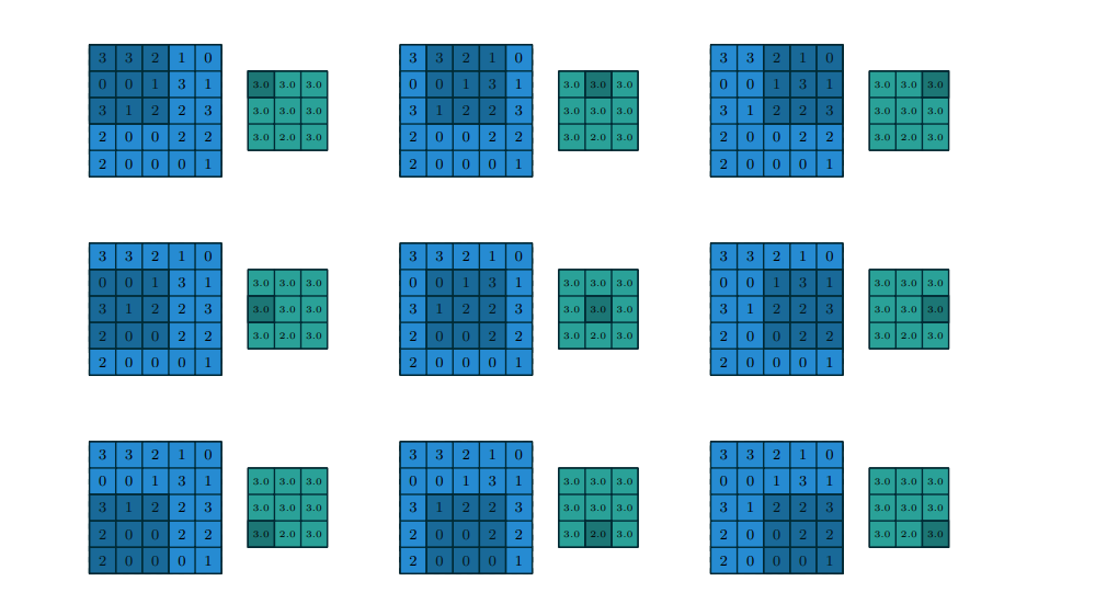
a 5 × 5 input using 1 × 1 strides.8
Average Pooling: This method calculates the average value of all elements within the defined region. It captures a summary of the feature information within that area.
[[10,  5,  8,  2],
 [12,  7,  3,  1],
 [15, 11,  6,  4],
 [ 9, 14, 13,  0]]

Similar to max pooling, slide the 2x2 filter across the feature map one step at a time (stride of 1).
For each position of the filter, calculate the average value of all elements within the region it covers.

Top-left position: Average of (10, 5, 12, 7) = (10 + 5 + 12 + 7) / 4 = 8.75
Top-right position: Average of (5, 8, 7, 3) = (5 + 8 + 7 + 3) / 4 = 6.75
Bottom-left position: Average of (12, 7, 15, 11) = (12 + 7 + 15 + 11) / 4 = 11.25
Bottom-right position: Average of (7, 3, 11, 6) = (7 + 3 + 11 + 6) / 4 = 6.75

Final output:
[[ 8.75,  6.75],
 [11.25,  6.75]]Code language: PHP (php)
As you can see, instead of taking the maximum value, average pooling calculates the average of all elements within the filter region. This provides a different kind of summary of the feature information in that area. It maintains a smoother representation of the feature information, incorporating contributions from all elements within the region. This can be helpful for tasks like image classification, where capturing a broader feature summary is beneficial.
- Pooling layers are often used after the activation function in a CONV layer.
- The size of the pooling filter (usually 2×2) and the stride (step size between filter applications) can be hyperparameters tuned during training to achieve optimal performance.
- Max pooling is generally more common than average pooling, as it tends to capture more robust features.
- You can experiment with stacking multiple pooling layers with different filter sizes or strides to extract features at various scales.
You can also achieve the same thing by using convolutional layers with bigger stride filters for down-sampling. The work by Springenberg et al. (2014) and the popular ResNet architecture demonstrate that strided convolutions can achieve good performance on various datasets, suggesting their viability as an alternative to pooling. Try out what works best for your project.
Fully Connected Layers
Additionally, you can also use multiple convolutional layers as hidden layers. This allows the network to extract progressively higher-level features from the image. After the final convolutional layers, the network typically transitions to fully-connected layers. This allows the network to integrate information from all extracted features and make a final prediction or classification decision based on the learned representation of the image.
While the majority of a CNN is composed of convolutional and pooling layers for feature extraction, FC layers are typically found towards the end of the network. After multiple convolutional and pooling layers, the spatial information is reduced, and the network captures local features. Here is what happens in FC layers in CNN:
1. Flattening the Input:
- Unlike convolutional layers that operate on 3D tensors (containing feature maps), FC layers require a 1D vector as input.
- The process of flattening involves transforming the output from the previous layer (typically a 3D tensor from the final convolutional layer or the pooling layer) into a single long vector.
- This vector essentially combines all the activations from the feature maps into a linear representation.
2. Matrix Multiplication: Each FC layer is essentially a mathematical operation involving two key components:
- Weight Matrix: This matrix contains learnable weights for each connection between neurons in the current layer and neurons in the previous layer (the flattened input vector).
- Bias Vector: This vector contains a bias term for each neuron in the current layer.
- The flattened input vector is multiplied by the weight matrix. This multiplication essentially combines the features extracted by the previous layers with learned weights.
3. Bias Addition: The bias vector is then added element-wise to the product obtained from the matrix multiplication. The bias term allows each neuron in the FC layer to shift its activation independently.
4. Non-linear Activation (Optional): In most FC layers, a non-linear activation function (like ReLU) is applied to the output after adding the bias. This introduces non-linearity into the network’s decision-making process, allowing it to learn more complex relationships between the features.
5. Repeated for Multiple Layers: Often, several FC layers are stacked one after another. Each layer performs the same basic steps (flattening, matrix multiplication, bias addition, activation), further transforming and integrating the features.
6. Output Layer: The final FC layer has an output size that depends on the task:
- Classification: The number of output neurons matches the number of classes the network is trying to predict. A Softmax activation function is typically used to convert the outputs into class probabilities (e.g., identifying cats and dogs in images).
- Regression: The output layer has a single neuron with a linear activation function to predict a continuous value (e.g., estimating the age of a person in an image).
So, essentially, this is how you can visualize our typical final CNN architecture in 3D:
My recommendation is to start seeing these operations in terms of matrices rather than 3D visualization because that way it is a lot easier to visualize what’s going on deep inside the model. Also, before you move ahead, I would recommend reading this paper.
CNN In Practice:
- https://www.corsi.univr.it/documenti/OccorrenzaIns/matdid/matdid950092.pdf ↩︎
- https://microscopy.unimelb.edu.au/__data/assets/pdf_file/0007/2796244/Fundamentals-of-digital-imaging-2018.pdf ↩︎
- Same as 1 ↩︎
- https://arxiv.org/pdf/1603.07285.pdf ↩︎
- https://arxiv.org/pdf/1603.07285.pdf ↩︎
- https://pyimagesearch.com/deep-learning-computer-vision-python-book/ ↩︎
- https://pyimagesearch.com/deep-learning-computer-vision-python-book/ ↩︎
- Same as 5 ↩︎
Amritesh Kumar
I believe you are not dumb or unintelligent; you just never had someone who could simplify the concepts you struggled to understand. My goal here is to simplify AI for all. Please help me improve this platform by contributing your knowledge on machine learning and data science, or help me improve current tutorials. I want to keep all the resources free except for support and certifications. Email me @amriteshkr18@gmail.com.
