Mathematics For Machine Learning: Mathematical Intuition Basics
Mathematics is the core of many sciences, including machine learning and data science. But how exactly does it help us solve such complex problems? What happens behind the scene that allows us to teach computers to perform tasks that seemed impossible decades ago? The answer lies in the power of mathematics, which provides the tools and frameworks needed to model, analyze, and solve these problems. In this tutorial on mathematics for machine learning, we will build mathematical intuition, exploring how core mathematical concepts drive the algorithms and techniques we use today. We will focus on the fundamentals as these concepts are often overlooked in machine learning courses, preventing learners from understanding the core principles behind the ML algorithms.
Understanding these concepts not only unlock (to some extent) the “black box” nature of machine learning models but also empowers us to make better decisions when designing and tuning them. Machine learning problems are often dealt with in n-dimensional space due to the nature of data, unlike the 2D or 3D spaces we commonly imagine. However, the concepts we learn for 2D space can be expanded to n-dimensional space, along with the intuition for what is happening. So, let’s start from scratch.
Table of Contents
Data – The Fuel Of Machine Learning Algorithms
Data is the main fuel that helps machine learning algorithms solve complex problems. By representing data such as images, audio, or text in numerical terms, we can perform mathematical operations on them. This is exactly what we do: first, we find a way to represent various data types using numbers, and then we apply mathematical algorithms to learn patterns.
Let’s consider a very simple tabular data. This data has a rows and columns. Each column represents a different feature of the data. Each row corresponds to an individual or a data point with specific values for each feature.
| Age | Height | Weight |
|---|---|---|
| 25 | 180 | 75 |
| 30 | 165 | 60 |
| 22 | 170 | 68 |
| 28 | 160 | 55 |
Each row of the table can be considered a single data point because it represents data for an individual person. However, we often perform operations collectively on each column to get an overall picture of the dataset. We can represent each column or row as a vector and perform calculations on them. By plotting these vectors, we can visualize their existence in space.
For example, if you take the “Age” column on the x-axis and the “Height” column on the y-axis, you can visualize the relationship between these two features. Similarly, you can take the “Weight” column on the z-axis and visualize the data points in a 3D space. In practice, however, we often deal with datasets containing many rows and columns, making it impossible to visualize the entire dataset in an n-dimensional space. Therefore, we typically select two or three columns for analysis.
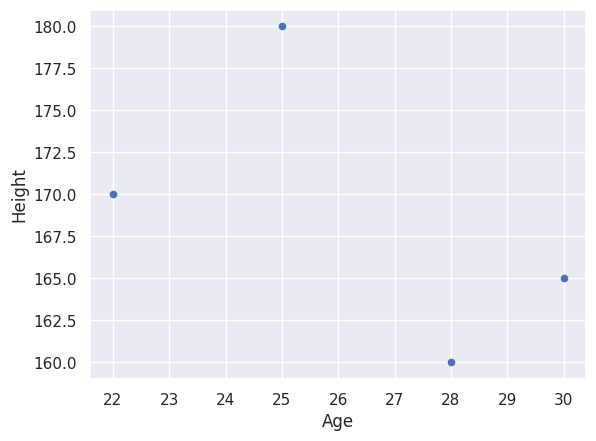
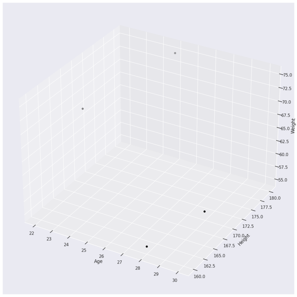
Although we conceptualize our data as existing in an n-dimensional space (e.g., 3D space in the case of three features), performing mathematical calculations efficiently on this data collectively is crucial. This is where matrices come into play. By representing the data in a matrix form—with rows as vectors of individual data points and columns as feature vectors—we can perform calculations on the entire dataset efficiently.
The entire dataset can be represented as a matrix, where each row is a vector (data point), and each column is a feature. This structure mirrors how data is often collected and organized in tables or spreadsheets.
[
 [25, 180, 75],
 [30, 165, 60],
 [22, 170, 68],
 [28, 160, 55]
]Code language: JSON / JSON with Comments (json)
Each row [25, 180, 75] is a data point, and each column represents a feature (Age, Height, Weight). Once, we have our data represented in matrix form, we can perform mathematical calculations. Operations on matrices can be efficiently performed using vectorization, a method where operations are applied to entire arrays or matrices at once rather than iterating over individual elements. This speeds up computations significantly compared to looping through each element.
A lot of things can be done once we have represented our data in matrix form. In neural networks, the weights and activations of neurons are represented as matrices, and operations on these matrices define the learning process. Matrices enable batch processing, where multiple data points can be processed simultaneously, improving computational efficiency and leveraging parallel processing capabilities. Techniques like Singular Value Decomposition (SVD) and Principal Component Analysis (PCA) rely on matrix operations to reduce dimensionality and extract meaningful features from the data. These things are possible because matrices have many beautiful properties.
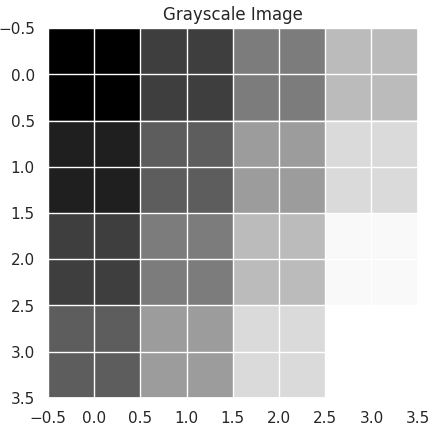
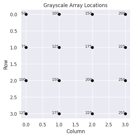
Similar to tabular data, images exist multidimensional space. A grayscale image is represented as a 2D array, where each element represents the intensity of a pixel. The values typically range from 0 (black) to 255 (white) for 8-bit images. Check the image below and see how as the value changes the color distribution changes as well. You can even plot the location of pixels on the graph.
[[ 50 100 150 200]
 [ 75 125 175 225]
 [100 150 200 250]
 [125 175 225 255]]

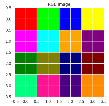
this is a 2D grayscale image matrixCode language: CSS (css)Similarly, you can have RGB images.
RGB Image Array:
[[[255   0   0]
  [  0 255   0]
  [  0   0 255]
  [255 255   0]]

 [[255   0 255]
  [  0 255 255]
  [255 165   0]
  [128   0 128]]

 [[  0 128   0]
  [128 128   0]
  [  0   0 128]
  [128   0   0]]

 [[  0 255 127]
  [255  20 147]
  [ 75   0 130]
  [255 140   0]]]Code language: CSS (css)
Tabular data features are typically structured and discrete, with clear semantic meanings. Image features, especially raw pixel values, are unstructured and represent visual information. These pixel values are the basic features of an image. For a grayscale image of 28×28 pixels (like in MNIST digit recognition), you have 784 features (28 x 28). For color images, each pixel has three values (one for each color channel: Red, Green, and Blue). So, for an image of 28×28 pixels, you have 784 pixels but 3 values per pixel, totaling 2352 features.
These pixels create more complex features. At a basic level, features can be simple patterns like edges (where the color changes significantly) or corners. For example, in facial recognition, the edges of eyes, nose, and mouth are important features. At a higher level, features can represent whole objects or significant parts of objects. In a neural network(CNN), early layers detect simple features like edges, while deeper layers detect complex features like eyes, wheels, or even entire faces. When an image is processed by a neural network, it creates feature maps that highlight where certain features (like edges or textures) are found in the image.
Audio signals can be represented as 1D arrays (wave-forms), 2D matrices (spectrograms), or even higher-dimensional representations like Mel-Frequency Cepstral Coefficients (MFCCs). Text data can be converted into numeric representations using methods like Bag of Words (BoW), Term Frequency-Inverse Document Frequency (TF-IDF), word embeddings, and sentence embeddings, discussed in another tutorial on NLP.
Fundamentally, data in various forms (text, images, audio) is first converted into a numeric format (using matrices or arrays) to enable calculations, analysis, and machine learning operations.
Mathematics For Machine Learning: Tools
Once data is converted into a numeric form, mathematics becomes a powerful tool to analyze, interpret, and make decisions based on that data. When working with data, we often aim to make informed decisions or uncover insights. To achieve these goals, we use various tools. Probability theory helps us make predictions by quantifying the likelihood of different outcomes based on our data.
Statistics enables us to analyze and interpret data, revealing patterns and hidden relationships. Since data in ML is frequently represented in matrices, linear algebra provides the necessary framework for performing complex operations on our data. Additionally, we also use calculus to deal with various calculations involved in these two fields. Overall, machine learning uses various mathematical tools not limited to these four fields.
The main area is statistics, which encompasses probability concepts. Linear algebra and calculus then follow, aiding in complex calculations. We will focus on statistics and probability here. Linear algebra is discussed in notes, and algorithm specific tutorials. Calculus is something you are expected to know, at least its basics.
Statistics Basics For Machine Learning
Imagine you’re a researcher trying to understand people’s coffee consumption habits in a large city. You’re interested in discovering not only how much coffee people drink but also the factors influencing their choices. First, let’s start with descriptive statistics. This involves collecting data and summarizing it to get an overview of what’s happening. For instance, you gather information about the average number of cups of coffee people drink daily, the most popular types of coffee, and the most frequented coffee shops. Descriptive statistics help you describe the current situation but don’t tell you about the underlying patterns or causes.
To dig deeper, we turn to inferential statistics, where we make predictions and draw conclusions about the broader population based on a sample. For example, based on the data from a subset of the city’s population, you might infer the coffee consumption habits of the entire city. Inferential statistics allow you to make educated guesses and predictions beyond the data you directly observe. Here the term population refers to all the coffee drinkers in the city.
However, it’s impractical to survey everyone, so you select a sample, a smaller group representative of the population. The characteristics you observe in the sample, like the average number of cups consumed per day, are called statistics. These statistics help estimate parameters, the true values in the entire population, such as the average coffee consumption across all city residents. In many machine learning problems, the goal is mainly to estimate population parameters or understand underlying patterns within a broader population based on the sample data.
As you collect data, you encounter different types of variables. Numerical variables are quantitative and represent numbers, such as the number of cups of coffee consumed or the price paid per cup. These can be further divided into discrete variables (like the number of cups, which you can count) and continuous variables (like the temperature of the coffee, which can take any value within a range). On the other hand, categorical variables classify data into different categories, such as coffee types (espresso, latte, cappuccino) or customer demographics (age groups, gender).
The data you gather can be qualitative or quantitative. Qualitative data refers to descriptive information that categorizes or labels attributes, such as customer satisfaction levels (good, fair, poor). Quantitative data involves numerical measurements, like the amount of coffee consumed. Within quantitative data, you distinguish between discrete (countable, like the number of visits to a coffee shop) and continuous (measurable, like the duration of each visit). You can summarize these using the mean (average cups consumed) or proportion (percentage of people preferring a certain type of coffee).
To ensure your sample accurately represents the population, you must carefully choose your sampling method. Random sampling gives every individual an equal chance of being selected, reducing bias. This can be done through:
- Simple random sampling, where you randomly select participants from the population.
- Stratified sampling, where you divide the population into groups (like age or income brackets) and sample from each group proportionally.
- Cluster sampling, where you divide the population into clusters (like neighborhoods) and randomly select entire clusters.
You might also use systematic sampling, where you select every nth individual from a list, or convenience sampling, where you choose participants who are easy to reach. However, convenience sampling can introduce sampling errors if the sample isn’t representative of the population. Additionally, errors can arise from factors unrelated to the sampling process, known as nonsampling errors, such as misreporting by participants.
Understanding the level of measurement is crucial for analyzing data accurately. The nominal scale level categorizes data without a specific order (like coffee types). The ordinal scale level arranges data in a meaningful order but without precise differences between ranks (like customer satisfaction ratings). The interval scale level allows for meaningful differences between data points but lacks a true zero (like temperature in Celsius – zero degrees Celsius doesn’t mean there’s no temperature; it’s just a reference point). The ratio scale level has all the features of the interval scale plus a true zero (for example, zero weight means there’s no weight at all), allowing for meaningful ratios (like weight or income).
When analyzing data, you might look at the frequency of different responses, the relative frequency (proportion of the total), or the cumulative frequency (running total of frequencies). For example, you might find that 40% of respondents drink coffee daily, representing the relative frequency, and track how these percentages accumulate as you move through different categories.
But how can we describe our data to get meaningful insights? We can get an understanding of our data by using a few things like mean, media and plots. Let’s understand them with examples.
Measures of the Location: Measures of location provide a way to understand the position of a particular value within the dataset. They are useful for understanding the distribution of data and identifying relative standings
Imagine you’re analyzing customer spending data for an online store. You want to understand where individual spending figures lie relative to the entire dataset. This involves several key concepts:
- Percentiles divide the data into 100 equal parts. For example, the 90th percentile indicates that a customer’s spending is higher than 90% of all customers. To find the 90th percentile, you sort all spending values in ascending order and identify the value below which 90% of the data falls.
- Median (although categorized under central tendency) is the middle value when all data points are sorted. If there’s an even number of data points, it’s the average of the two middle values. The median provides a central value that’s not skewed by extreme outliers.
- Quartiles split the data into four equal parts. The first quartile (Q1) is the 25th percentile, the second quartile (Q2) is the median (50th percentile), and the third quartile (Q3) is the 75th percentile. The interquartile range (IQR) is the difference between Q3 and Q1 and measures the spread of the middle 50% of the data.
Outliers are values significantly different from the majority. You can detect them using the IQR: values beyond Q1 – 1.5 * (IQR) and Q3 + 1.5 * (IQR) are often considered outliers.
In machine learning, percentiles and quartiles help in understanding the distribution of features. For instance, if you’re dealing with customer income data, the 25th percentile might show the lower end of the income distribution, and the 75th percentile the upper end. This helps in creating features that capture customer segmentation.
Unlike the mean, which can be heavily influenced by extreme values (outliers), the median provides a more robust measure of central tendency. This is particularly useful in datasets with skewed distributions or outliers. When normalizing or standardizing data, the median can be used instead of the mean to center data, especially in the presence of outliers. For example, using median-based centering can make your data preprocessing more robust. The median can be used to impute missing values in continuous features. This is often preferred over the mean when the data contains outliers or is skewed.
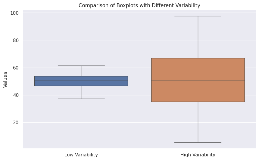
Box-whisker plots (or box plots) can be used to graphically analyze these values. The box represents the Interquartile Range (IQR), which covers the middle 50% of the data. The top and bottom edges of the box are the third quartile (Q3) and first quartile (Q1), respectively. A line inside the box indicates the median (Q2), which divides the dataset into two equal halves. It’s the 50th percentile. The whiskers extend from the edges of the box to the smallest and largest values within 1.5 * IQR from the quartiles. They show the range of the data excluding outliers. Any data points beyond this range are considered outliers and are often plotted as individual points.
If the median line is centered within the box, the data is symmetrically distributed. If it’s skewed towards one side, the data may be skewed. A larger box indicates more variability in the middle 50% of the data. A shorter box indicates less variability.
Measures of Center: (Also known as measures of central tendency) Measures of center provide an indication of the general location of the data points, giving a sense of where the data tends to cluster.
- Mean is the average of all data points. For instance, if you have customer spending data of $100, $150, and $200, the mean is ($100 + $150 + $200) / 3 = $150. It provides a measure of central tendency but can be affected by outliers.
- Mode is the most frequently occurring value. If most customers spend $100, the mode is $100. It’s useful for understanding the most common spending level.
- Median is the middle value and is less affected by outliers compared to the mean. If customer spending data is $100, $200, and $5000, the median is $200, giving a better sense of central tendency when data is skewed.
The mean is sensitive to extreme values (outliers) because it takes into account every value in the dataset. In skewed distributions, the mean tends to be pulled towards the longer tail, hence it shifts in the direction of the skewness. The median is the middle value that divides the dataset into two equal parts. It is less sensitive to outliers and skewed values because it only depends on the order of values. In skewed distributions, the median is located between the mean and the mode. The mode is the most frequently occurring value in the dataset. In skewed distributions, the mode represents the peak or the highest point in the distribution and is typically unaffected by extreme values.
Since it is often impossible to measure the mean of entire population, statisticians rely on the sample mean to estimate the population mean. The population mean (μ) is constant for a given population. The sample mean varies depending on the sample taken (x̄).
Measures of Spread: They describe the extent to which data points in a dataset vary or differ from each other. Unlike measures of central tendency, which focus on locating the center of the data, measures of spread provide insight into the variability and dispersion within the dataset.
At its core, the idea of measuring spread arises from the need to quantify how scattered or concentrated the data points are around a central value. This concept is crucial because two datasets may have the same mean or median but can differ significantly in how their values are distributed. For example, in quality control, understanding variability is as important as knowing the average; a process with high variability might still produce defective items, even if the average quality is high.
Imagine a factory that produces metal rods with a target length of 100 cm. The acceptable tolerance range is between 99.5 cm and 100.5 cm. If the process produces rods with lengths ranging from 98 cm to 102 cm, this indicates high variability. While the average length might still be 100 cm, the range shows that some rods are significantly outside the acceptable limits, leading to a high defect rate.
The most basic measure of spread is the range, which is calculated as the difference between the maximum and minimum values in the dataset. The range provides a simple measure of the total spread of the data but is sensitive to extreme values or outliers, which can distort the true variability of the dataset. Despite its limitations, the range is useful for a quick, rough estimation of data dispersion.
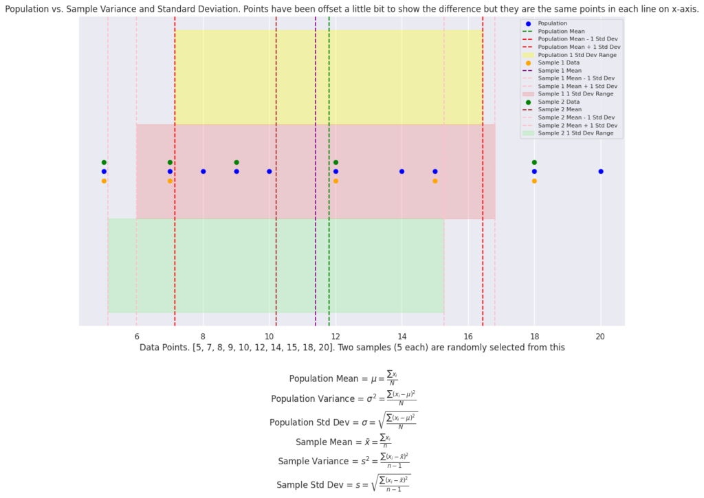
A more sophisticated measure of spread is the variance, which quantifies the average squared deviation of each data point from the mean. The idea of squaring the deviations arises from the desire to eliminate the issue of positive and negative deviations canceling each other out. By squaring these differences, we ensure that all deviations contribute positively to the overall measure, thus providing a meaningful sense of the data’s variability. The variance provides a comprehensive picture of the data’s spread but comes with the drawback of being in squared units of the original data, making it less intuitive to interpret directly.
To address the interpretability issue of variance, the standard deviation was introduced. The standard deviation is the square root of the variance, bringing the measure back to the same units as the original data. This adjustment makes the standard deviation a more intuitive measure of spread, as it directly relates to the original data’s scale. The standard deviation indicates the average distance of data points from the mean, providing a clear and practical sense of variability. The theoretical basis for these measures lies in the desire to understand not just the typical or average behavior of data but also the extent to which individual observations deviate from this norm.
When we have data from an entire population, we calculate the variance by finding the average of the squared deviations from the mean. A deviation is the difference between a data point and the mean. To get the variance, we square these deviations (to avoid negative values canceling out the positive ones), sum them up, and then divide by the total number of data points, N.
When we only have a sample from the population, we need to account for the fact that a sample might not capture all the variability present in the entire population. To correct for this potential underestimation, we divide by n−1 instead of n, where n is the sample size.This adjustment, called Bessel’s correction, compensates for the tendency of a sample variance to underestimate the population variance. By dividing by n−1, we ensure that our estimate is unbiased.
Now that we have a some intuition of these basic concepts related to descriptive statistics. Let’s talk about probability that will help understand more advance concepts related to statistical inference. Probability theory provides the foundation for statistical inference. Statistical methods often rely on probability distributions to model and analyze data.
Probability Basics For Machine Learning
The concept of probability started to take shape with the work of French mathematician Blaise Pascal and Italian mathematician Gerolamo Cardano. Cardano, in the 16th century, explored probability in gambling and games of chance. In the 17th century, Pascal’s correspondence with Pierre de Fermat laid the foundation for probability theory. They discussed problems related to gambling and formed the basis of modern probability theory. The 18th century saw further formalization by mathematicians like Abraham de Moivre and Jakob Bernoulli, who developed key principles of probability and laid the groundwork for statistical theory.
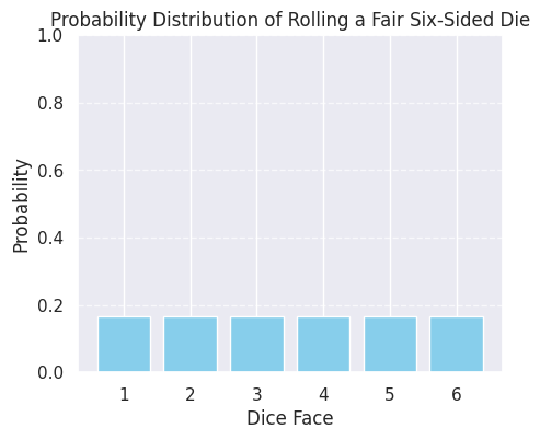
First, let’s talk about an experiment. Think of an experiment as a controlled process or activity where you observe outcomes. For example, let’s say you’re rolling a six-sided die. This action of rolling the die is an experiment. It’s planned and controlled because you decide when and how to roll the die, but the result (which number shows up) is not predetermined—it’s a matter of chance. If the result of an experiment isn’t due to chance, it’s typically a deterministic process rather than a probabilistic one. This means that the outcome is entirely predictable given the initial conditions.
An outcome is what you get as a result of an experiment. When you roll a die, the outcome could be any one of the numbers from 1 to 6. Each roll produces one specific number, and that’s the outcome of that roll. The outcome should not be predictable with certainty before conducting the experiment. There should be an element of chance involved as mentioned above. In a probabilistic experiment, outcomes must be equally likely. This means that each outcome is just as likely to happen as any other outcome.
The idea of equally likely outcomes simplifies probability calculations and helps us understand certain types of experiments better. The experiment must have a well-defined sample space, which is the set of all possible outcomes. This helps in calculating probabilities. Additionally, the experiment should be repeatable under the same conditions. This means you should be able to perform the experiment multiple times and observe outcomes that align with the defined sample space.
An event is a collection of outcomes that you’re interested in. Let’s say you want to know the probability of rolling an even number. The event here is “rolling an even number,” which includes the outcomes 2, 4, and 6. So, the event is just a way to group together specific outcomes that match what you’re interested in. The sample space is like a complete list of all possible outcomes of an experiment. For rolling a die, the sample space includes every number the die could land on: {1, 2, 3, 4, 5, 6}. It’s the full set of all possible outcomes you could get from the experiment.
An “or” event in probability refers to the situation where either one event, the other event, or both events occur. It is also known as the union of two events. An “and” event in probability refers to the situation where both events occur simultaneously. It is also known as the intersection of two events. Disjoint events, also known as mutually exclusive events, are events that cannot occur at the same time. In other words, if one event happens, the other cannot (simultaneously).
Probabilities are proportions of a whole. Probability theory is built on a set of foundational rules, known as axioms. These axioms are basic principles that define how probabilities work. Non-Negativity: Probabilities are always positive or zero. This means that the likelihood of an event is never negative. Normalization: The total probability of all possible outcomes must add up to 1. Additivity: If you have two or more disjoint events that cannot occur at the same time, the probability of either event occurring is the sum of their individual probabilities.
Sometimes we want to know to know the probability of an event given another event has already occurred. In that case, we calculate conditional probability. Conditional probability is a measure of the probability of an event occurring, given that another event has already occurred. The conditional probability of event A given that event B has occurred, denoted as P(A|B), is defined as: P(A|B) = P(A ∩ B) / P(B). P(A∩B) is the probability that both A and B happen. All properties of probability discussed above remain valid for this as well.
Now what happens if the knowledge of B does not affect the chance of event A? In that case, A will be an independent event. This means, P(A|B) = P(A ) or P(A ∩ B) = P(A)P(B). If you are wondering if disjoint events are independent then the answer is “no”. Disjoint simply means they cannot happen simultaneously (A ∩ B is zero) . This does not mean the occurrence of one event does not affect the probability of another, if one happens the other does not.
This (A ∩ B | C) = P(A|C) P(B|C), is called conditional independence. Two events are conditionally independent given a third event if knowing whether the second event has occurred does not change the probability of the first event once the third event is known. Independence does not imply conditional independence, and vice versa.
Sometimes, we have multiple events, and if each pair of these events are independent to each other we call that pairwise independence. Pairwise independence does not imply that the events are mutually independent because the condition of independence should be satisfied for all possible intersections, including all events which may not be the case.
Now, imagine you’re trying to determine the likelihood of raining tomorrow, but you have different weather forecasts. Each forecast has its own probability of being correct and gives a different prediction for rain. Total probability theorem combines these probabilities to give an overall chance of rain by accounting for each forecast’s likelihood and its prediction. P(A) = P(A|B1) * P(B1) + P(A|B2) * P(B2) + … + P(A|Bn) * P(Bn), where Events B1, B2, B3…represent different weather forecasts and Event A is the event of it raining tomorrow.
Another important concept that you will come across is Bayes’ Rule. Conceptually, it flips the relationship between cause and effect. If we know the probability of an effect given a cause, Bayes’ rule helps us determine the probability of the cause given the effect. Let’s say we have n possible causes, H1, H2, …, Hn, and an observed effect E. The probability of Hi given E is: P(Hi | E) = (P(E | Hi) * P(Hi)) / Σ[P(E | Hj) * P(Hj)] for j = 1 to n. By combining your initial belief (prior probability) with the likelihood of observing the new evidence given your belief, Bayes’ rule provides a way to calculate your updated belief (posterior probability).
These were just the basics from your high school mathematics. Now let’s move forward.
Some Advance Basics:
While outcomes represent the possible results of an experiment, they often lack a numerical representation that’s convenient for mathematical operations and analysis in real world applications. This is where random variables come into play. A random variable is essentially a numerical representation of an outcome. It assigns a numerical value to each possible outcome of a random experiment. This transformation allows us to use mathematical tools and techniques to analyze and understand the data. So, here is how we can differentiate:
Outcomes are the fundamental results of a random experiment. For instance, when flipping a coin, the outcomes are heads or tails. Events are a collection of one or more outcomes. For example, getting a head when flipping a coin is an event. Random Variable on the another hand is a function that assigns a numerical value to each outcome. For instance, we can define a random variable X as follows: X = 1 if the outcome is heads, and X = 0 if the outcome is tails.
There are two types of random variables: Discrete(countable number of distinct values – the number of heads when flipping three coins. Possible values are 0, 1, 2, or 3) and Continuous (an infinite number of values within a given range – the height of a person, which can be any value within a certain range).
Once we’ve assigned numerical values to the outcomes of a random experiment using a random variable, we can delve deeper into understanding the likelihood of these values occurring. This is where probability distributions come into play. Essentially, it’s a function that maps the values of the random variable to their corresponding probabilities.
We have two main ways to describe probability distributions: Probability mass functions or PMFs for the discrete case, and PDFs or probability distribution(density) functions for the continuous random variable case. Instead of assigning probabilities to individual values, a PDF represents the probability density at a particular point. The total area under the PDF curve equals 1, indicating the total probability of all possible values. It’s important to note that the probability of a specific value for a continuous random variable is actually zero; instead, we consider probabilities over intervals.
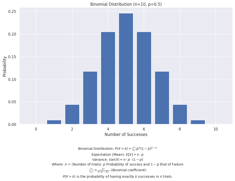
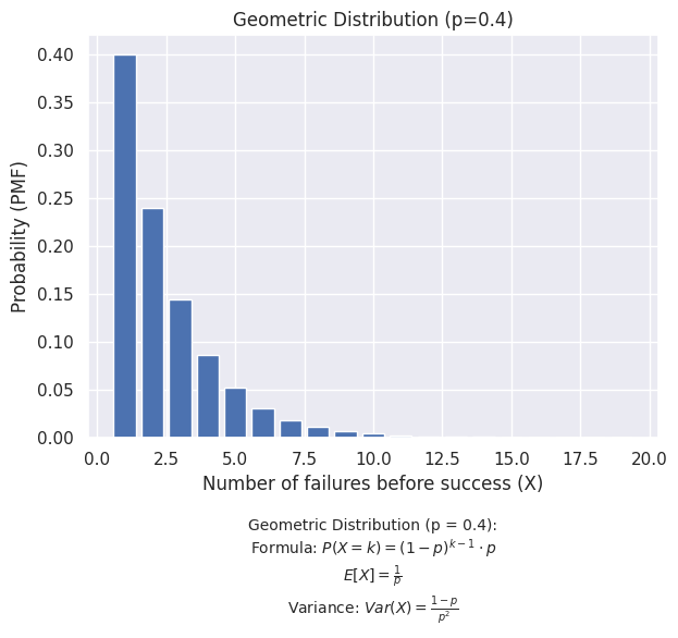
Let’s see how it looks like when plot the PMFs and PDFs:
Read the captions of the above plots to get an idea of what it means to be PMFs and PDFs. Once we have the distribution of a random variable, we can employ the concepts we’ve learned to extract valuable insights or summarize the random variables. One such concept is Expectation which is similar to mean but used mostly in context of PMFs and PDFs.
Expectation (or Expected Value) is a fundamental concept that provides a measure of the “central tendency” of a random variable. It represents the average value that the random variable is expected to take if an experiment were repeated many times. In both cases (PMFs, and PDFs), the expectation is essentially a weighted average of all possible values, with the weights being the probabilities associated with those values. Similarly we can use variance etc to describe our random variable. You can find the equations here.
Now, what can we do with probability distributions? Various problems in probability tend to have a distribution that we can use to perform calculations and solve our problems.
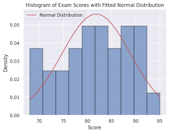
Note that, PDFs are not the same as data distributions. PDFs don’t represent real-world data but rather an idealized or theoretical representation of how data might be distributed. Data distributions are empirical representations of how data is actually distributed in a dataset. They are derived from real-world observations and measurements. While they can often be approximated by PDFs, they are not identical. Data distributions may have irregularities, outliers, or specific patterns that don’t perfectly match any theoretical distribution.
By fitting a probability distribution to data, we construct a theoretical model that approximates the data’s underlying pattern. This model, often represented by a curve or equation, allows us to estimate probabilities, make predictions, identify anomalies, and draw statistical inferences.
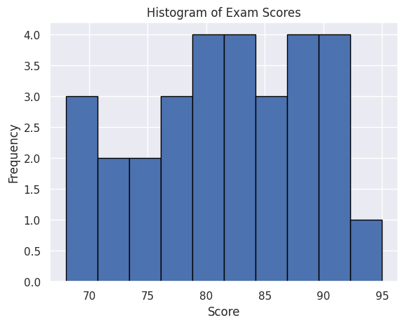
Empirical data can be visualized using distributions such as Histogram, Bar Chart, etc. but there are various types of probability distributions that exist for each case (discrete and continuous) design for various types of problems. Let’s look at them one by one.
Discrete Case(PMFs) – Probability Mass Functions:
A Bernoulli trial is a simple experiment with only two possible outcomes: success or failure. Think of flipping a coin – heads could be success, and tails would be failure. Each trial is independent, meaning the outcome of one trial doesn’t affect the next. This also means the probability of success remains the same for each trial. We will use this in next few explanations. All points are valid for them as well.
The Bernoulli distribution is one of the simplest and most fundamental probability distributions. It models the outcome of a single Bernoulli trial. If you put n = 1 in the binomial distribution explain below, and you will get the Bernoulli distribution.
A binomial distribution is a probability distribution that models the number of successes in a fixed number of independent Bernoulli trials. For instance, flipping a coin ten times and counting the number of heads follows a binomial distribution. Key characteristics include a fixed number of trials (n), a constant probability of success (p) for each trial, and independent trials. The outcomes of a binomial experiment fit a binomial probability distribution.
Geometric distributions are used to model the number of trials needed to achieve the first success in a sequence of Independent Bernoulli trial. A unique property of the geometric distribution is its memorylessness. This means that the probability of the next success doesn’t depend on the number of failures that have already occurred.
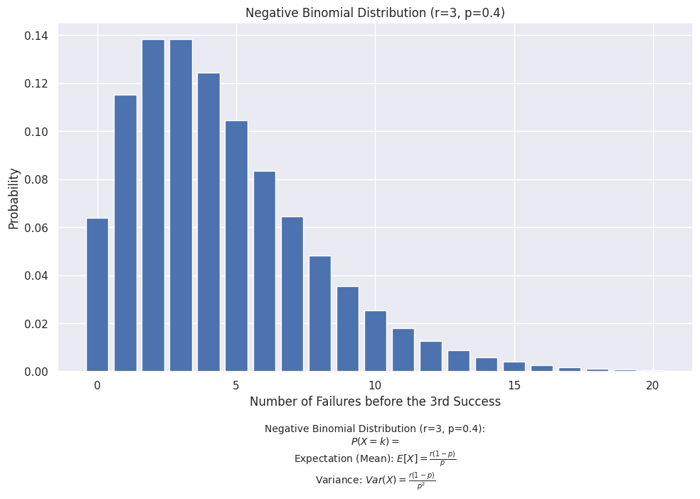
This above distribution is closely related to another distribution called the negative binomial distribution, which models the number of failures before a specified number of successes occur in a sequence of Independent Bernoulli trial. Since the probability of the next success is influenced by how many successes you’ve already accumulated, it does not have memorylessness property.
The Poisson distribution models the number of events occurring in a fixed interval of time or space when these events happen independently of each other at a constant average rate.Let’s say a call center receiving incoming calls. The exact timing of each call is unpredictable, but on average,the center receives a certain number of calls per hour. This scenario is well-suited for a Poisson distribution. It models the number of events (incoming calls – even if it is rare like 2-3 calls) occurring within a fixed interval (an hour) when the events happen independently at a constant average rate. If mutations in a segment of DNA occur with an average rate of 0.5 mutations per cell, the number of mutations observed in a large sample of cells can be modeled using the Poisson distribution, despite mutations being rare events.
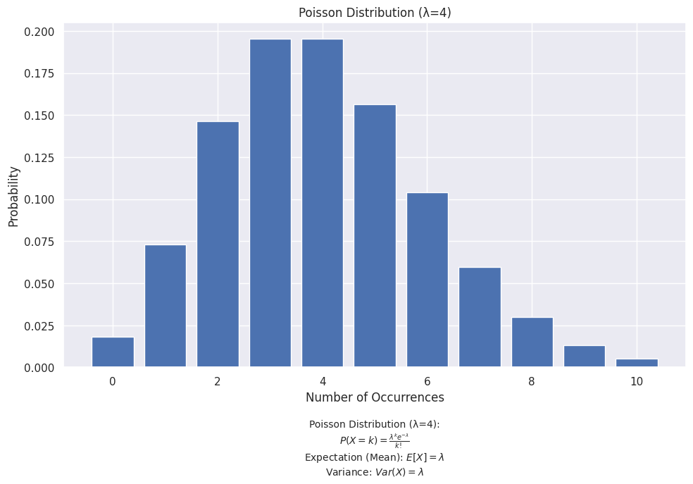
When the number of trials is vast and the probability of success is minuscule, the distribution of the number of successes approximates a Poisson process, where events occur independently and randomly at a constant rate. As n grows larger and p becomes smaller, with λ = n⋅p constant, the binomial distribution approximates the Poisson distribution.
The multinomial distribution is a generalization of the binomial distribution to more than two possible outcomes. It models the number of occurrences of each outcome in a fixed number of trials, where each trial results in one of several possible outcomes. A simple example is when you roll a fair die 10 times, and you want to model the number of times each of the 6 faces appears. Unfortunately, it is difficult to plot the PMFs. For more information read this.
There are other distributions too but the above mentioned distributions are the most common in discrete case. Feel free to explore further. The core thing is you just need to find a distribution that fits your problem, and understand the goal behind what it means by probability distribution.
Continuous Case(PDFs) – Probability Density Functions:
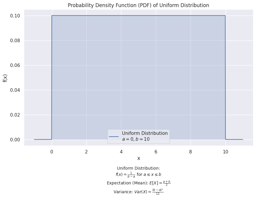
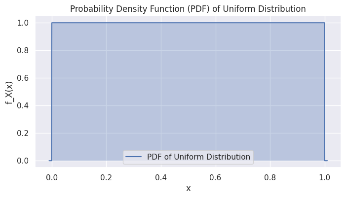
The uniform distribution is one of the simplest continuous probability distributions. It describes a situation where all outcomes in a given range are equally likely. It can be discrete as well.
The PDF f(x) gives the density of probability at a particular point x in the continuous interval. Unlike discrete distributions where the height represents the probability of a specific outcome, in continuous distributions, the height does not represent the probability directly but rather the density. The “density” at a particular point x indicates how concentrated (more likely) the probability is around that point, but it does not represent the probability of X = x directly.The total area under the curve is 1. The probability can be found by calculating the area under the curve between two points. The probability that a continuous random variable equals any specific value is zero. Instead, we talk about the probability of the variable falling within a range.
The PDF f(x) of a continuous random variable can take on values greater than 1, but this doesn’t mean that the probability at any specific point is greater than 1 because probabilities are associated with intervals, not specific points.
The exponential distribution is often used to model waiting times between independent events that happen at a constant rate. For example, it can describe the time until a radioactive particle decays, the time until a customer arrives at a service point, or the time between earthquakes in a region. A key characteristic of the exponential distribution is its memoryless property.
This means that the probability of an event occurring in the future is independent of how much time has already passed. In other words, if you’ve been waiting for a bus for 10 minutes, the probability of the bus arriving in the next 5 minutes is the same as if you had just started waiting. This property is unique to the exponential distribution and has significant implications for its applications. The exponential distribution is defined by a single parameter, lambda (λ), which represents the average rate of events. A higher value of λ indicates that events happen more frequently (shorter waiting times), while a lower λ means events occur less frequently (longer waiting times).
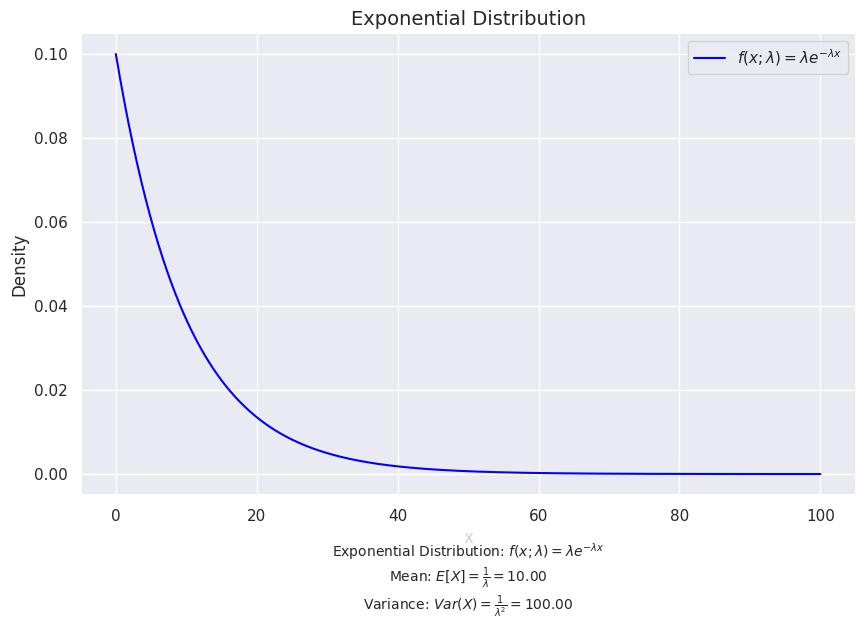
λ = 0.1. The curve shows the probability density, which decreases as x increases. This reflects the fact that short waiting times are more likely, while long waiting times are less likely. The mean is E[X] = 10. This represents the average time you would wait for an event (e.g., the next bus) to occur. The exponential distribution is skewed to the right, meaning it has a longer tail on the right side. This reflects the fact that while short waiting times are common, there is also a possibility of very long waiting times.
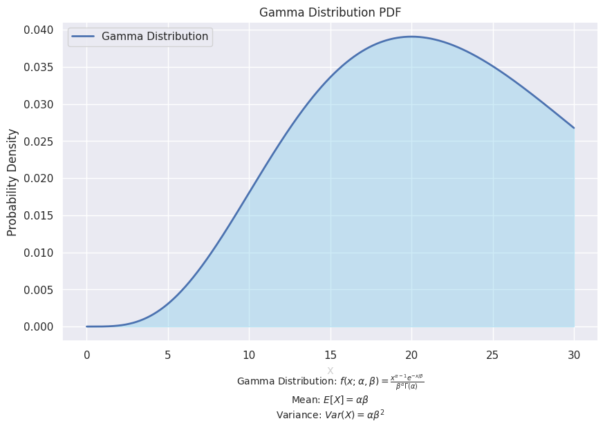
The Gamma distribution is a two-parameter family of continuous probability distributions, which generalizes the exponential distribution. It is often used to model the time until an event occurs k times (where k is not necessarily an integer). This distribution has two parameters. Shape and scale parameters. You will also come across rate parameter which is nothing but inverse of scale parameter.
The shape parameter, often denoted by α or k, controls the shape of the Gamma distribution. In the context of a Poisson process, the shape parameter of Gamma distribution can be interpreted as the number of events you are waiting for. For instance, if α=3, the Gamma distribution models the waiting time until three events have occurred. The value of α influences the skewness and mode of the distribution: If α < 1: The distribution is highly skewed to the right. If α = 1: The distribution is an exponential distribution. For α > 1, the distribution is skewed right but becomes more symmetric as α increases.
The rate parameter, denoted by λ controls the rate at which events occur in the Poisson process. It is the reciprocal of the scale parameter (θ). The rate parameter represents the average number of events per unit time. A larger λ results in a steeper, more compressed distribution (shorter waiting times), while a smaller λ results in a flatter, more spread-out distribution (longer waiting times).
The scale parameter, denoted by θ or β is the reciprocal of the rate parameter. It controls the scale or spread of the distribution. It represents average waiting time. These parameters allow the Gamma distribution to model a wide range of phenomena, from highly skewed distributions to more symmetric ones. For example, if you are monitoring a server, and the requests to the server follow a Poisson process with an average of λ = 0.2 requests per second or β = 5 . You might want to model the time until you receive 5 requests. The waiting time for these 5 requests can be modeled by a Gamma distribution with α=5 and λ=0.2.
The Beta distribution is a continuous probability distribution defined on the interval [0, 1] or (0, 1). This makes it particularly useful for modeling probabilities themselves. It’s characterized by two positive shape parameters, typically denoted as α (alpha) and β (beta). These parameters control the shape of the distribution. Intuitively, the Beta distribution can be thought of as representing the distribution of probabilities. For example, if you’re uncertain about the true probability of success of a coin flip, you might model your belief about this probability using a Beta distribution.
One of the key strengths of the Beta distribution is its flexibility. By varying the values of α and β, you can create a wide range of shapes, from highly skewed distributions to nearly uniform ones. This makes it a versatile tool for modeling various phenomena. Read this for more.
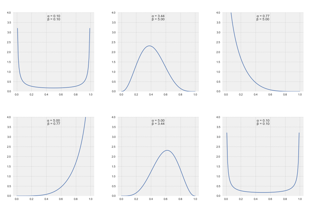
A conjugate prior is a special type of prior distribution that makes this updating process mathematically convenient. It ensures that the posterior distribution belongs to the same family as the prior distribution. For the Binomial likelihood, the Beta distribution is the conjugate prior. This means that if you start with a Beta prior and update it with Binomial data, the posterior distribution will also be a Beta distribution. This property simplifies the process of updating beliefs with new data, making the Beta distribution a convenient choice for modeling probabilities in Bayesian inference.
Before we go ahead to the one of the most important PDFs used in machine learning, we should not skip a few things:
Cumulative Distribution Functions (CDFs): As you move along the x-axis (values of the random variable), the CDF tells you the accumulated probability up to that point. In other words, the value of the CDF at a particular point helps to determine the proportion of the probability distribution that lies below that point. It can exist for both Continuous and Discrete case.
A joint distribution describes the probability of two or more events occurring simultaneously. It provides a comprehensive view of how these variables interact with each other and how their joint behavior can be quantified. For discrete random variables X and Y, the joint PMF is denoted as: P(X = x, Y = y) = f(x, y), where f(x, y) is the probability that X takes the value x and Y takes the value y simultaneously. The marginal PMF of X is obtained by summing the joint PMF over all possible values of Y: P(X = x) = Σ_y P(X = x, Y = y)
For continuous random variables X and Y, the joint PDF is denoted as: fX,Y(x,y). For continuous random variables X and Y, the probability of X falling between a and b, and Y falling between c and d is given by the double integral of the joint probability density function (PDF) over that region: P(a ≤ X ≤ b, c ≤ Y ≤ d) = ∬[a,b]x[c,d] fX,Y(x,y) dy dx. For more details read this.
The marginal distribution of a subset of variables within a joint distribution focuses on the probability distribution of those specific variables, disregarding the others. It simplifies the analysis by providing insights into the behavior of individual variables independently of their joint behavior with other variables
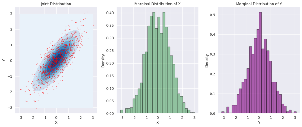
You will also hear about conditional distributions which describe the probability distribution of one or more random variables given that other variables are fixed at certain values. In the context of joint distributions, the conditional distribution provides insights into how one variable behaves when another variable is known or constrained to a specific value. It help understand how the distribution of one variable is influenced by the value of another variable.
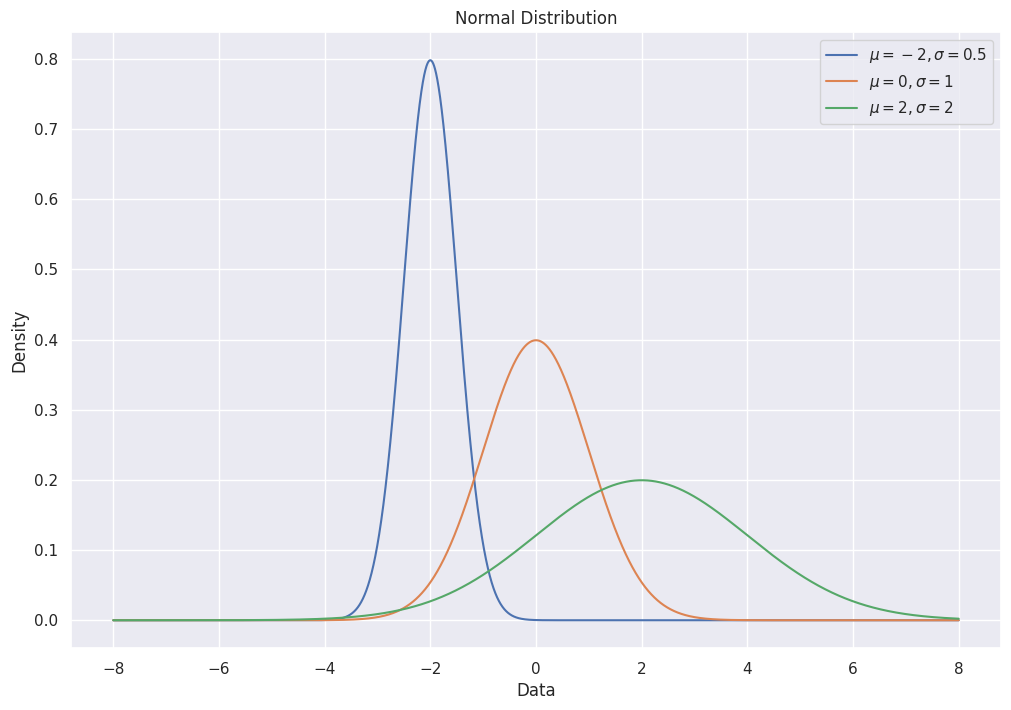
Now let’s come to the Normal Distribution or Gaussian distribution, which is the most important one for machine learning. The normal distribution is a continuous probability distribution characterized by its bell-shaped curve. It is defined by two parameters: the mean (μ) and the standard deviation (σ). The mean represents the center of the distribution, while the standard deviation determines its spread. It is symmetric around the mean and area under the curve is 1. Shifting μ to the right or left moves the entire curve without changing its shape. A larger σ results in a flatter, wider curve, while a smaller σ produces a taller, narrower curve.
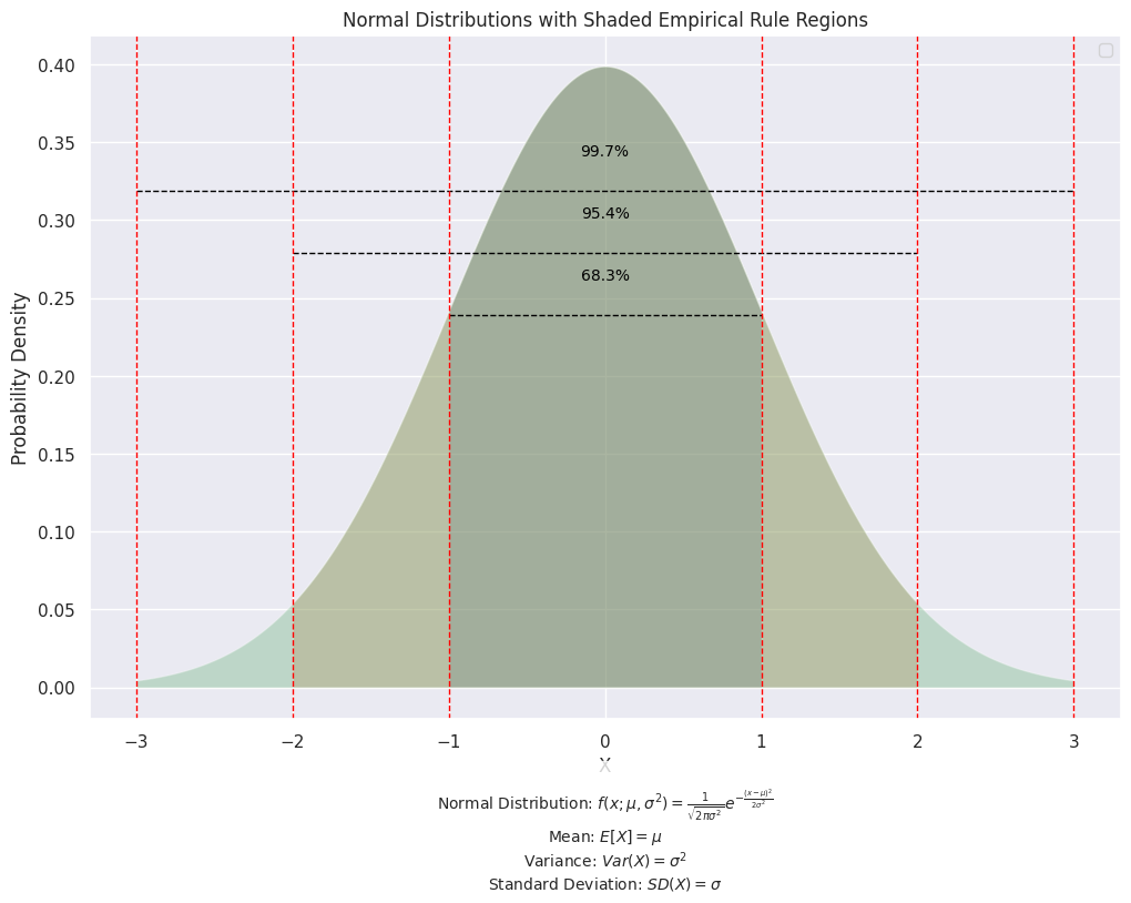
Now, what if we want to compare values from two different normal distributions. In that case, we can use z-scores. A z-score, represents the number of standard deviations a data point is from the mean of its distribution. z = (x – μ) / σ, where x is a raw value. For instance, a Z-score of 2 means the data point is 2 standard deviations above the mean. Z-scores standardize data to have a mean of 0 and a standard deviation of 1. This makes it easier to compare data points from different distributions. The standard normal distribution is a special case of the normal distribution with a mean of 0 and a standard deviation of 1. The CDF of the standard normal distribution gives the probability that a normally distributed random variable is less than or equal to z.
Z-scores can help identify outliers. A data point with a Z-score greater than 3 or less than -3 is typically considered an outlier, as it lies far from the mean.
Many machine learning algorithms assume normally distributed data. Creating new features in a dataset based on normal distributions can improve model performance. Algorithms like Linear Regression, Logistic Regression, and Gaussian Naive Bayes often rely on the assumption of normally distributed data or error. Gaussian Mixture Models (GMMs) use multiple normal distributions to model complex data distributions. Deviations from normality can indicate outliers or anomalies in the data. When evaluating machine learning models, performance metrics (such as accuracy or error rates) can be analyzed using normal distribution assumptions to understand variability and confidence intervals.
The Central Limit Theorem:
In machine learning, you will often hear the term IID which means Independent and Identically Distributed. Independent means, the observations or data points are not correlated or connected to each other. Identically distributed means that all observations come from the same probability distribution.
Suppose you’re training a machine learning model to classify emails as spam or not spam. You collect a dataset of 1,000 emails, and you label each one as either spam or not spam. If these emails are IID, it means: Whether one email is spam or not does not affect whether another email is spam. All emails are drawn from the same population, meaning the process that generates these emails (and their labels) is consistent throughout the dataset.
When training a model, the IID assumption ensures that the data you’re using to train the model is representative of the underlying process you want to model. This helps in generalizing from the training data to unseen data. The IID assumption is crucial for making valid statistical inferences. It allows for the use of central limit theorems, which underpin the construction of confidence intervals and hypothesis tests. The IID assumption helps in estimating the model’s performance on unseen data. For example, cross-validation assumes that the training and validation sets are IID, ensuring that performance estimates are unbiased.
If the data is not identically distributed (e.g., if the training data comes from a different distribution than the test data), the model’s estimates can be biased. This might lead to poor generalization on new data. If the data points are not independent, the model might overfit or underfit.
Now let’s consider an example, Imagine you love coffee and every morning, you buy a cup from your favorite coffee shop. You’ve noticed that the time it takes you to get your coffee varies a bit every day, sometimes it’s 3 minutes, sometimes 5 minutes, but it’s always around 4 minutes on average. Now, let’s say you start timing how long it takes every day. On day one, it takes 4.5 minutes. On day two, it’s 3.8 minutes. You keep recording, and over time, as you gather more and more data, the average of all your recorded times starts getting closer and closer to that 4-minute mark.
This is what we call convergence—as you collect more observations (more days), the average time it takes to get your coffee converges to the true average (in this case, 4 minutes). Now suppose you only recorded the time for 5 days. The average might be a bit off—maybe 4.2 minutes or 3.9 minutes. But what if you recorded it every day for a whole year? After 365 days, you would expect the average time to be very close to 4 minutes. This is the Law of Large Numbers (LLN) in action. The LLN tells us that as the number of observations increases, the average of those observations will get closer to the true average.
There are two types of LLN:
- Weak Law of Large Numbers (WLLN): This version assures you that if you keep recording, the average will eventually be very close to 4 minutes, but not necessarily right away. It might still fluctuate a bit as you keep counting.
- Strong Law of Large Numbers (SLLN): This is an even stronger statement, saying that if you could keep recording forever (infinite days), the average would not just get close to 4 minutes—it would actually settle down exactly at 4 minutes and stay there.
The above explanation however is too oversimplified.
The LLN is why we trust averages. Even if you see some variation in the short term, in the long run, you can expect the average to represent the true value accurately. The SLLN states that the sample average will almost surely converge to the expected value as the sample size approaches infinity. In practical terms, this means that the probability of the sample average not converging to the true mean is zero.
Let’s take another example for this, let’s say you’re flipping a fair coin. You know that in theory, you should get heads 50% of the time. But if you flip it only 10 times, you might get 7 heads and 3 tails, which is 70% heads. That seems far from 50%! However, the LLN tells us that if you keep flipping that coin many, many times – let’s say thousands or even millions of times – the percentage of heads you get will get closer and closer to 50%. It’s like the more data you collect, the more accurate your results become. The Weak Law says that as you increase your number of coin flips, the chance of your result being far from 50% gets smaller and smaller. The Strong Law makes an even bolder claim. It says that if you could flip the coin infinitely many times, your result would definitely settle exactly at 50%.
I have provided some mathematical equations here but you can refer to this resource or this one for more rigorous understanding.
Now, let’s come back to the original example and say you’ve got the average time it takes to get your coffee (4 minutes), but you’re also curious about the distribution of all those times you recorded. Maybe most days it’s around 4 minutes, but sometimes it’s much quicker, and occasionally it takes much longer. Here’s where the Central Limit Theorem (CLT) comes in.
CLT tells us that if you were to take lots of samples (like averaging the times over different weeks), the distribution of those sample averages would form a bell-shaped curve, known as a normal distribution, regardless of how the original times are distributed. For example, you randomly pick 30 days out of the year, calculate the average time it took to get coffee on those days, and then repeat this process many times. The CLT tells us that the histogram of these averages would look like a bell curve centered around 4 minutes.
The CLT is why the normal distribution (the bell curve) is so common in statistics and machine learning. Even if the data itself isn’t normally distributed, the averages of samples taken from that data often are. This is why normal distribution assumptions are often reasonable in real-world applications.
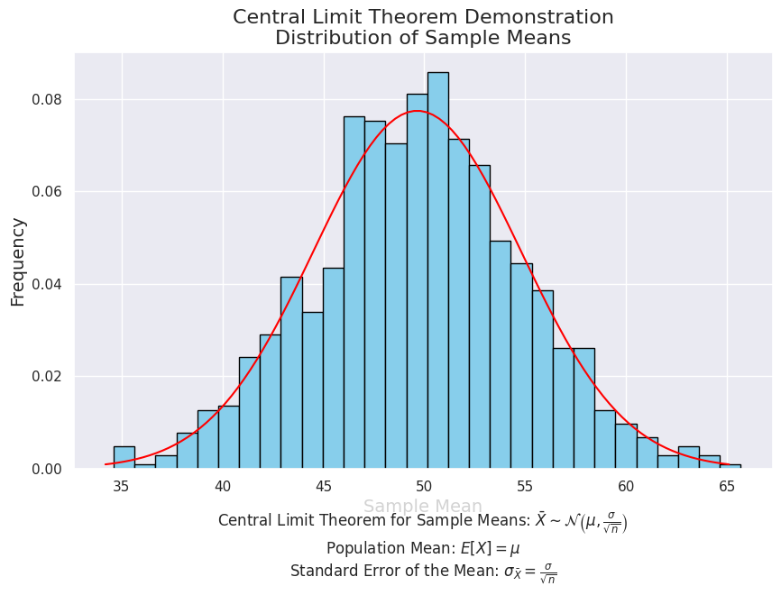
and calculate their means, these sample means form a new distribution called the sampling distribution of the mean which describes the distribution of these sample means. The mean of the sampling distribution of the mean is the same as the mean of the original distribution. The variance of the sampling distribution of the mean is the variance of the original distribution divided by the sample size n. The standard deviation of the sampling distribution of the mean, called the standard error of the mean (SEM), is the square root of the variance. This is a measure of how much the sample mean is expected to vary from the population mean.
You just need sufficient number of samples each of size typically greater than or equal to 30 to see this in practice.
Confidence Intervals And Hypothesis Testing:
Now that we’ve discussed the Central Limit Theorem (CLT), let’s discuss the concept of confidence intervals, which is closely related. The Central Limit Theorem tells us that the distribution of sample means will approximate a normal distribution as the sample size grows, regardless of the population’s distribution. This powerful result allows us to make inferences about population parameters, such as the mean, using sample data. This is called statistical inference which provides methods for drawing conclusions about a population from sample data.
A confidence interval is a range of values, derived from a sample, that is likely to contain the population parameter (like the population mean) with a certain level of confidence. In other words, it’s a way of saying, “We are X% confident that the true population mean lies within this interval.” For example, suppose we calculate a 95% confidence interval for the mean height of adult males in a certain region. If the interval is [170 cm, 180 cm], we are saying that we are 95% confident that the true mean height of all adult males in that region lies between 170 cm and 180 cm.
Confidence Level is the probability that the confidence interval actually contains the true population parameter. Common confidence levels are 90%, 95%, and 99%. It’s crucial to understand that a confidence interval is not a probability statement about the population parameter itself. Instead, it reflects the reliability of the estimation process. If we were to repeat the sampling process many times, we would expect about 95% of the calculated confidence intervals to contain the true population mean.
Let’s understand this using an example. Let’s say you’re trying to estimate the average height of adult women in a city. You randomly select 100 adult women from the city and measure their heights. You find the average height of these 100 women and calculate the standard deviation. Using the sample mean, standard deviation, sample size, and desired confidence level (e.g., 95%), you calculate the confidence interval. This gives you a range of values where you believe the true population mean height lies. If you repeated this process many times (i.e., took many different samples of 100 women), you would find that approximately 95% of the confidence intervals you construct would contain the true average height of all adult women in the city.
Confidence is about the interval, not the population parameter: We are confident that the process of constructing confidence intervals will capture the true population parameter 95% of the time. Each individual interval either contains the true mean or it doesn’t. We don’t know for sure whether a specific interval captures the true mean. Increasing the sample size generally leads to narrower confidence intervals, providing a more precise estimate of the population parameter.
In practice, we usually only have one sample, and from that single sample (it’s often impractical in real-world scenarios due to time, cost, and resource constraints to deal with multiple samples that’s why we should try our best to get a sample that is representative of the population), we estimate the population parameter. The confidence interval accounts for the fact that our estimate is based on just one sample, so it gives us a range where the true parameter is likely to be.
The standard error is a measure of how much the sample mean is likely to vary from the true population mean. It quantifies the sampling error. Standard Error (SE) = Population Standard Deviation (σ) / Square Root of Sample Size (n). A larger sample size reduces the standard error, meaning the sample mean is more likely to be closer to the population mean. A larger population standard deviation increases the standard error, indicating more variability in the data. If you’re measuring the heights of adults, the standard error of the mean height would be smaller for a sample of 1000 people than for a sample of 100 people.
Now we wil use the concept from CLT. In practice, you usually take just one sample, and you calculate one sample mean. Even though you have just one sample, the CLT allows you to use the properties of the normal distribution to create a confidence interval around the sample mean.
The CLT states that as the sample size increases, the distribution of the sample mean (x̄) approaches a normal distribution, even if the original population distribution is not normal. For large sample sizes (typically n>30), the sampling distribution of the sample mean is approximately normal, regardless of the population distribution. The Z-score is a value that tells us how many standard deviations a particular data point (or, in this case, the sample mean) is from the mean of a standard normal distribution (which has a mean of 0 and a standard deviation of 1). The Z-score is used because it allows us to standardize our data, making it easier to calculate probabilities and confidence intervals. For example, a Z-score of 1.96 corresponds to a 95% confidence level, meaning that 95% of the values lie within 1.96 standard deviations from the mean in a standard normal distribution. Similarly, a Z-score of 2.58 corresponds to a 99% confidence level.
By multiplying the standard error by the critical value (in our case Z-score) which helps define the width of the confidence interval, we determine the margin of error. This margin is then added and subtracted from the sample mean to create the confidence interval.
The margin of error determines the width of a confidence interval. It’s the amount added and subtracted from the sample mean to create the interval’s upper and lower bounds. Margin of Error (ME) = Critical Value * Standard Error. A larger margin of error means a wider confidence interval, indicating more uncertainty. A smaller margin of error means a narrower confidence interval, indicating less uncertainty. If you want a 95% confidence interval and have a standard error of 2, and the critical value (z-score) is 1.96, the margin of error would be 1.96 * 2 = 3.92.
Now, let’s see how we can calculate confidence interval:
The first step is to decide how confident you want to be that your interval contains the true population parameter (e.g., the population mean). Common choices are 90%, 95%, and 99%. The confidence level determines the critical value you’ll use. Next, calculate the mean of your sample. This is your best estimate of the population mean. Calculate the standard error which gives you a sense of how much the sample mean might vary from the population mean. Look up the critical value for your chosen confidence level in their respective table. Calculate margin of error which is found by multiplying the critical value by the standard error. Finally, add and subtract the margin of error from the sample mean to get the confidence interval.
Example 1: In this example, we are assuming that we know the population standard deviation but in most real world scenario we don’t know this. When we know the standard deviation of population we assume normality.
A researcher wants to estimate the average IQ of adults in a certain population.
A random sample of 100 adults is selected, and their IQ scores are measured.
The sample mean IQ is found to be 100, and the population standard deviation is known to be 15.
Construct a 95% confidence interval for the population mean IQ.

Given:
Sample mean (x̄) = 100
Population standard deviation (σ) = 15
Sample size (n) = 100
Confidence level = 95%

Steps:

1. Find the z-score: For a 95% confidence level, the z-score is 1.96.
2. Calculate the standard error:SE = σ / √n = 15 / √100 = 1.5
3. Calculate the margin of error (E):E = z * SE = 1.96 * 1.5 = 2.94
4. Construct the confidence interval:
     Lower limit = x̄ - E = 100 - 2.94 = 97.06
     Upper limit = x̄ + E = 100 + 2.94 = 102.94

Interpretation:
We are 95% confident that the true population mean IQ lies between 97.06 and 102.94.Code language: JavaScript (javascript)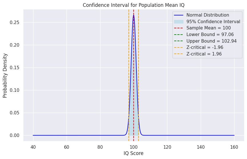
Example 2: We can also find sample size for a population Mean
Let's say we want to estimate the average height of adult males in a city with a 95% confidence interval
and a margin of error of 2 inches.Assuming a population standard deviation of 3 inches,
we can use the following formula: n = (Z * σ / E)^2

n is the sample size
Z is the z-score for the desired confidence level (1.96 for 95%)
σ is the population standard deviation
E is the margin of error

n = (1.96 * 3 / 2)^2 = 8.4649
We would round up to 9, meaning we need a sample size of 9 males to achieve the desired level of precision.
In real life you may also need to consider other factors instead of relying on the formula alone.
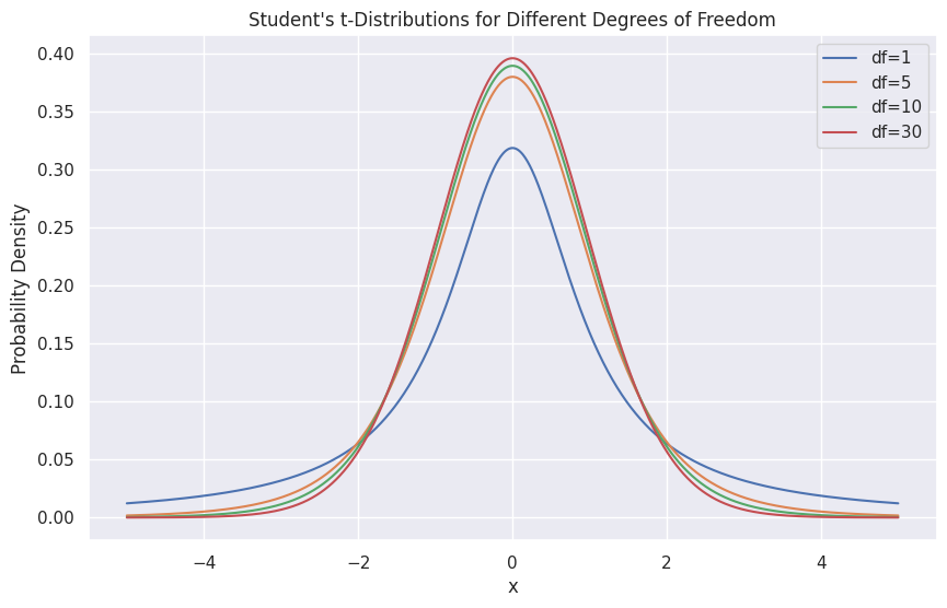
When sample size is too small, we use t-distribution, instead of normal distribution especially when population standard deviation is not known. Even if you have bigger sample size but population standard deviation is not know then use t-distribution. The t-distribution is similar to the standard normal distribution but has fatter tails. This means it accounts for more variability and is more robust to outliers or deviations in small samples.
The shape of the t-distribution is determined by its degrees of freedom, which is equal to the sample size minus one (n-1). As the sample size increases, the t-distribution approaches the normal distribution. This is because with larger sample sizes, the estimate of the population standard deviation becomes more reliable. For very large sample sizes, the difference between the t-distribution and normal distribution becomes negligible.
When calculating confidence intervals, if the population standard deviation (σ) is known, we use the normal distribution and standard normal critical values (z). However, if σ is unknown, we estimate it using the sample standard deviation (s) and use the t-distribution instead, also when sample size is very small. In this case, the confidence interval is calculated by first computing the standard error (SE) as SE = s / √n. We then find t-scores or t-critical values using the degrees of freedom and the confidence interval. in the above example, you simply have to replace these values. You can also use confidence interval to calculate population proportions. The concept is the same. Feel free to read about the same.
Here is a function to calculate the confidence interval for both the cases:
import numpy as np
from scipy import stats

def confidence_interval(data, confidence_level, distribution = "t-distribution"):
    mean = np.mean(data)
    # standard error of mean
    sem = stats.sem(data)
    confidence_level = confidence_level/100 # to convert to decimal format
    degrees_of_freedom = len(data) - 1
    cumulative_probability = (1 + confidence_level) / 2
    if distribution == "t-distribution":
        critical_value = stats.t.ppf(cumulative_probability, degrees_of_freedom)
    elif distribution == "normal":
        critical_value = stats.norm.ppf(cumulative_probability)
    else:
        raise ValueError("Unsupported distribution. Choose 't-distribution' or 'normal'.")
    margin_of_error = critical_value * sem
    lower = mean - margin_of_error
    upper = mean + margin_of_error
    return float(round(lower, 2)), float(round(upper, 2))

if __name__ == "__main__":
        data = np.array([10, 12, 14, 16, 18, 20, 22])

        ci_normal = confidence_interval(data, 95, distribution="normal")
        ci_t_distribution = confidence_interval(data, 95, distribution="t-distribution")
        #ci_other = confidence_interval(data, 99, distribution="other") # willraise ValueError

        # Print results
        print("Confidence Interval using Normal Distribution:", ci_normal)
        print("Confidence Interval using T-Distribution:", ci_t_distribution)
        #print("Result for Unsupported Distribution:", ci_other)
Code language: Python (python)
In machine learning you can use confidence interval to understand the variability of evaluation metrics across different subsets of data. Confidence intervals can be used to quantify the uncertainty of predictions made by a model. This is particularly useful in regression tasks where you want to provide a range of likely values for a prediction. In cross-validation, confidence intervals can help to understand the variability of model performance metrics across different folds of the data.
Building on the idea of confidence intervals, which give us a range of values where we think a population parameter might fall, hypothesis testing comes into play when we want to make decisions or draw conclusions based on data. While a confidence interval tells us how uncertain we are about an estimate, hypothesis testing helps us decide whether the evidence in our data is strong enough to support a specific claim about the population.
Let’s say you’re thinking about buying a house and are curious about whether the property value in the area is really increasing, as some people say.
- Confidence Interval: You gather data on recent sales in the neighborhood and find that the average increase in property values over the past year is between $10,000 and $30,000. This confidence interval gives you an idea of how much home prices might have risen, with some uncertainty.
- Hypothesis Testing: Now, you want to be sure that this increase isn’t just due to random fluctuations in the market. Hypothesis testing helps you figure out if the observed increase is significant or if it might just be a temporary blip. You might test the hypothesis that there has been no real increase in property values and see if your data strongly suggests otherwise. If the test supports the idea that property values are genuinely rising, you might feel more confident in your decision to buy.
But how can we calculate it? In order to do that, we need to understand a few things. We start with two contradicting hypotheses. We then gather the data to check if it offers enough evidence to reject one of the hypotheses. Let’s understand these two Hypotheses.
First is null hypothesis (H0). The null hypothesis is like the “status quo” or the default assumption that nothing has changed or that there’s no effect. If you’re trying a new coffee recipe, and you want to know if it really tastes better than your usual one. The null hypothesis is the assumption that the new recipe tastes exactly the same as your old one. In other words, nothing special is happening—everything is as it has always been.
The second is alternative hypothesis(Ha). It is the idea that challenges the status quo. It’s what you’re trying to prove or support with evidence. In the coffee example, the alternative hypothesis would be that the new recipe actually does taste better. It’s the claim that something is different or has changed for the better.
When you perform a hypothesis test, you start by assuming the null hypothesis is true (the new coffee is no better than the old one). You then gather evidence (like taste-test results) to see if there’s enough proof to reject the null hypothesis in favor of the alternative hypothesis (that the new coffee is better). If your evidence is strong enough, you reject the null hypothesis and accept the alternative hypothesis, meaning you believe the new coffee is indeed tastier. If the evidence isn’t strong enough, you stick with the null hypothesis, concluding that the new coffee might not be better after all.
Once you have determined that your data supports one of these you make a decision in terms of whether to reject the null hypothesis or not. In hypothesis testing, we use different distributions depending on the specifics of our data and what we know about the population. When testing a single population mean, we either use a normal distribution or a Student’s t-distribution.
If we know the population standard deviation and the sample size is large enough, we use the normal distribution (often called a z-test). This is because, with a large sample size, the sample mean tends to be normally distributed, even if the population distribution itself isn’t perfectly normal. However, if the population standard deviation is unknown and we’re working with a smaller sample size, we use the Student’s t-distribution (called t-test).
For large samples (typically, n > 30 is considered sufficient), using the z-test is generally appropriate, even if the population standard deviation is unknown. The z-test and the t-test will yield very similar results in this case because the t-distribution approaches the normal distribution as the sample size increases. When dealing with large sample sizes, hypothesis testing becomes robust to deviations from normality in the population distribution. This means you can confidently use the normal distribution for inference as long as your sample size is large enough.
One of the key concepts in hypothesis testing is the level of significance, which is closely tied to the idea of confidence intervals. When we perform hypothesis testing, we’re often trying to determine whether the sample data provides enough evidence to reject a null hypothesis in favor of an alternative hypothesis. The level of significance, denoted by α, is a crucial component of this process. It represents the threshold at which we decide whether the evidence is strong enough to reject the null hypothesis. In simpler terms, the level of significance is the probability of making a Type I error, which occurs when we reject the null hypothesis even though it is actually true. For example, if we set α = 0.05, we are accepting a 5% chance of incorrectly rejecting the null hypothesis.
The level of significance is closely related to the confidence level used in confidence intervals. For instance, a 95% confidence interval corresponds to a 5% level of significance. This means that if we were to construct a 95% confidence interval for a population parameter and then conduct a two-tailed hypothesis test at a 5% significance level, the hypothesis test would reject the null hypothesis if the value specified by the null hypothesis falls outside of the confidence interval.
Another important concept is p-value. The p-value is a probability that measures the strength of the evidence against the null hypothesis. It represents the probability of obtaining a test statistic at least as extreme as the one observed, assuming that the null hypothesis is true. In simpler terms, the p-value tells us how likely our sample data would be if the null hypothesis were correct.
If the p-value is less than the significance level (p < α), we reject the null hypothesis. This means the evidence is strong enough to conclude that something other than chance is at play. If the p-value is greater than the significance level (p > α), we fail to reject the null hypothesis. This means the evidence is not strong enough to conclude that something other than chance is at play.
Example 3: Hypothesis testing
Imagine you are a data analyst at a company that runs a website.
The company claims that the average session duration on their website is 15 minutes.
However, you suspect that the average session duration might actually be different from 15 minutes.
To test this, you collect a random sample of session durations.
You start by setting up your null and alternative hypotheses:
NullHypothesis (H<sub>0</sub>): The average session duration is 15 minutes.
Mathematically, this is expressed as H<sub>0</sub>:μ =15 minutes.
Alternative Hypothesis (H<sub>a</sub>): The average session duration is not 15 minutes.
This is expressed as H<sub>a</sub>:μ≠15 minutes.
Choose a significance level:
You decide to use a significance level of α =0.05
This means you are willing to accept a 5% chance of rejecting the
null hypothesis when it is actually true (Type I error).
You collect data from a random sample of 30 sessions on the website.
After recording the session durations, you find that the sample has the following characteristics:
Sample size (n): 30
Sample mean: 14.5 minutes
Sample standard deviation (s): 2 minutes
Since the population standard deviation is unknown and the
sample size is relatively small, you use a t-test to compare the sample mean to the hypothesized population mean.
You can find the value of test statistics using the formula discussed earlier.
To find the p-value, you need to look up the t-value in a t-distribution table. Make sure to find degrees of freedom.
p-value will come out to be 0.18 (2 twice the value as it is two tailed.Check below) which is more than the value of alpha.
You compare the p-value to your significance level.
Since the p-value is greater than 0.05, you fail to reject the null hypothesis.
Failing to reject the null hypothesis means that there is not enough
evidence to support the claim that the average session duration is different from 15 minutes.
In other words, based on this sample, you do not have sufficient evidence to conclude that the
true average session duration is different from 15 minutesCode language: HTML, XML (xml)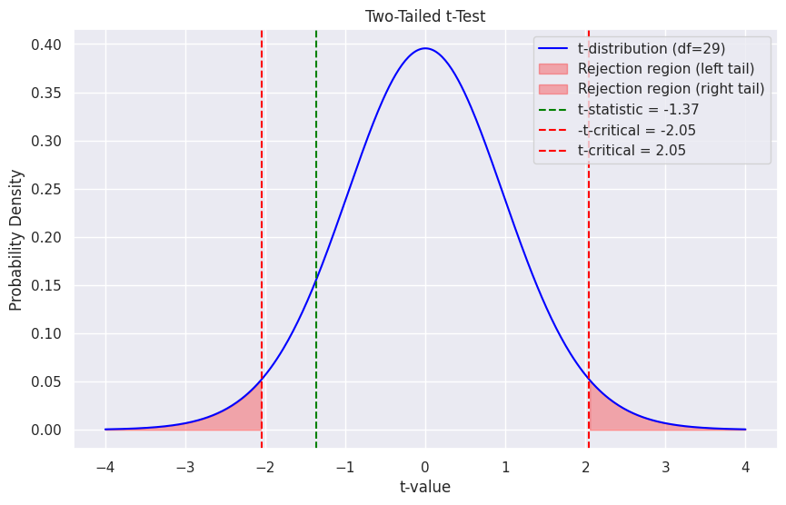
While performing the hypothesis testing you will have a few situations:
- You are interested in whether the parameter is either greater than or less than a certain value. In this case, the rejection region is located on the both end of the graph, and it is called two-tailed test. This means you’re looking at the possibility of an extreme outcome on either end of the distribution, which requires you to split your significance level (e.g., 5%) between both tails (2.5% in each tail). For example, if you’re testing whether a new drug has a different effect from the existing drug, you would use a two-tailed test because you want to know if the new drug is either more or less effective than the current one. In this case, the null hypothesis might state that the effectiveness of both drugs is the same, while the alternative hypothesis would state that the effectiveness is different, without specifying a direction.
- A one-tailed test is used when the alternative hypothesis specifies a direction of the effect—either greater than or less than a certain value, but not both. One-tailed tests are further classified into left-tailed and right-tailed tests, depending on whether you’re looking for a decrease or an increase. Left-Tailed Test: This is used when the alternative hypothesis suggests that the parameter is less than the null hypothesis value. For instance, if you want to test whether a new process reduces the average production time compared to the current process, you would use a left-tailed test. Here, the rejection region is in the left tail of the distribution. Right-Tailed Test: This is used when the alternative hypothesis suggests that the parameter is greater than the null hypothesis value. For example, if you’re testing whether a new marketing strategy increases sales, you would use a right-tailed test. The rejection region in this case is in the right tail of the distribution.
In hypothesis testing the decisions can be either correct or incorrect, leading to two types of errors:
- A Type I error occurs when we reject a null hypothesis that is actually true. The probability of committing a Type I error is denoted by alpha (α). Researchers typically set a small value for alpha (e.g., 0.05) to minimize the chance of this error.
- A Type II error occurs when we fail to reject a null hypothesis that is false. The probability of committing a Type II error is denoted by beta (β). 1 – β. is called the power of a test is the probability of correctly rejecting a false null hypothesis.
import numpy as np
from scipy import stats
import math

def hypothesis_test(data, h_mean, alpha = 0.05, axis=0, side = "two-sided"):

    """Performs a one-sample t-test to determine if the sample data significantly differs from a hypothesized population mean.

      Args:
          data: The sample data.
          h_mean: The hypothesized population mean.
          alpha: The significance level (default: 0.05).
          axis: The axis along which to compute the mean (default: 0).
          side: The alternative hypothesis ('two-sided', 'less', or 'greater').

      Returns:
          None
      """

    if side not in ["two-sided", "less", "greater"]:
        raise ValueError("Allow value for tails: two-sided, less, greater")

    t_statistic, p_value = stats.ttest_1samp(data, popmean = h_mean, axis = axis, nan_policy="omit", alternative = side)

    print(f"Calculated t-statistic: {t_statistic}")
    print(f"P-value: {p_value}")
    print(f"Significance level at {alpha}")

    if p_value < alpha:
        print("Reject Null Hypothesis")
    else:
        print("Fail to reject the null hypothesis")


if __name__ == "__main__":
    data = [2.5, 2.7, 3.1, 3.2, 2.8]
    h_mean = 3.0
    hypothesis_test(data, h_mean, axis = 0, side="greater")
Code language: Python (python)
The idea of hypothesis testing discussed above can become more clear with practice but one can also use the same approach if you want to test it for the two means when the population standard deviation is not know.
When comparing two population means and the population standard deviations are unknown, we employ a two-sample t-test or Welch’s t-test or Aspin-Welch t-test. This test determines if there’s a statistically significant difference between the means of two independent groups. The core idea is to assess whether the observed difference between the sample means is likely due to random chance or if it reflects a genuine difference between the population means.
Null hypothesis (H₀): There is no difference between the population means (μ₁ = μ₂). Alternative hypothesis (Hₐ): There is a difference between the population means (μ₁ ≠ μ₂, or μ₁ > μ₂, or μ₁ < μ₂ depending on the test).
The t-statistic for comparing two independent means is calculated as:

t = (x̄₁ - x̄₂) / √((s₁²/n₁) + (s₂²/n₂))

where:

    x̄₁ and x̄₂ are the sample means of the two groups
    s₁ and s₂ are the sample standard deviations of the two groups
    n₁ and n₂ are the sample sizes of the two groupsCode language: JavaScript (javascript)
The degrees of freedom for this is more complex than for a single-sample t-test. It involves using the Welch-Satterthwaite approximation , which is beyond the scope of this basic explanation. Most statistical software will calculate the degrees of freedom automatically. Based on the chosen significance level (α) and degrees of freedom, determine the critical t-value(s).
If the calculated t-statistic falls in the rejection region (beyond the critical values), reject the null hypothesis. Otherwise, fail to reject the null hypothesis. Alternatively, calculate the p-value associated with the calculated t-statistic and compare it to the significance level. The assumptions for the two-sample t-test include independence of the two samples and approximately normal distributions for the populations (or large sample sizes).
In hypotheis testing, we often come across a special type of distribution called chi-square distribution. The shape of the chi-square distribution is determined by its degrees of freedom. The chi-square distribution is formed by summing the squares of independent standard normal random variables.
- Start with a standard normal random variable Z, which has a mean of 0 and a standard deviation of 1.
- Square the standard normal variable Z. The result, Z2, is a chi-square distribution with 1 degree of freedom. This squaring process removes the symmetry of the standard normal distribution, leading to a distribution that only takes positive values and is skewed to the right. Now, if you have k independent standard normal random variables and you sum their squares, the resulting sum follows a chi-square distribution with k degrees of freedom. This k represents the number of independent pieces of information (or variables) contributing to the chi-square statistic.
The shape of the chi-square distribution is determined by its degrees of freedom. As the degrees of freedom increase, the distribution becomes less skewed and more symmetric, approaching a normal distribution as df becomes large. The chi-square distribution is defined only for non-negative values. Since it is the sum of squared normal variables, all values in the distribution are positive or zero.
The mean of the distribution equals its degrees of freedom, and the variance is twice the degrees of freedom. This relationship shows that as the degrees of freedom increase, both the mean and variance increase. One of the key properties of the chi-square distribution is that the sum of two independent chi-square distributed variables is also chi-square distributed, with the degrees of freedom being the sum of their individual degrees of freedom. The distribution has a long right tail, especially for small degrees of freedom. This property is why the chi-square distribution is often used to model the distribution of test statistics under the null hypothesis in hypothesis testing.
The shape of the chi-square distribution is unimodal, with the mode (peak) shifting to the right as the degrees of freedom increase. In hypothesis testing, critical values from the chi-square distribution table are used to determine whether to reject the null hypothesis. These critical values depend on the degrees of freedom and the chosen significance level (e.g., 0.05).
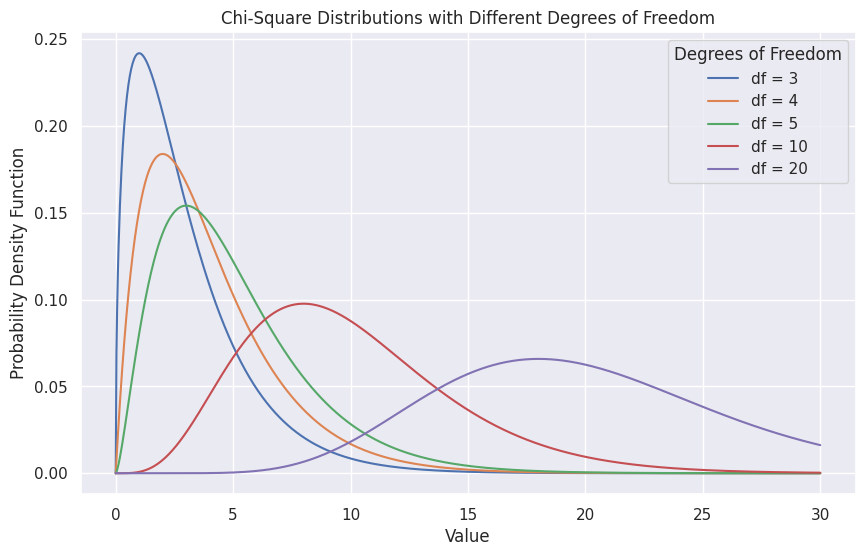
Now, there various types of hypothesis tests that can be done using this distribution:
Goodness-of-Fit Test: The goodness-of-fit test is a statistical method used to determine how well a set of observed values matches the values expected under a particular theoretical distribution. In essence, it helps us assess if our data aligns with a specific probability distribution. The chi-square test is a common statistical tool used for this purpose.
Consider you’re working on a machine learning classification problem where you’re predicting customer churn (whether a customer will leave a service). Suppose you build a model and classify customers into “churn” or “no churn” categories. After running the model, you want to evaluate whether the distribution of predicted churn rates matches the actual observed rates in your data.
- Define: Observed Frequencies: The actual count of customers categorized as “churn” and “no churn” in the test data.Expected Frequencies: The predicted count of customers in each category based on the model’s churn rate and the total number of customers. For example, if there are 1000 customers and the model predicts a 20% churn rate, we expect 200 churned customers and 800 non-churned customers.
- The chi-square statistic is calculated using the formula: χ² = Σ((Oi – Ei)² / Ei). Where χ² is the chi-square statistic. Oi is the observed frequency for a category. Ei is the expected frequency for the same category. χ² = ((250-200)²/200) + ((750-800)²/800) = 15.625.
- The degrees of freedom (df) for a goodness-of-fit test is calculated as: df = number of categories – 1. Which will be 1 in our case.
- Using a chi-square distribution table, find the critical value for the calculated degrees of freedom and a chosen significance level (e.g., α = 0.05). If the calculated chi-square statistic is greater than the critical value, reject the null hypothesis. For df = 1 and α = 0.05, the critical value is approximately 3.841. Since the calculated χ² (15.625) is greater than 3.841, we reject the null hypothesis, indicating that the predicted churn distribution doesn’t match the observed distribution.
Ensure that the expected frequencies in each category are not too small (typically, each should be 5 or more). If they are, the test results may not be accurate. Similar approach can be followed by another test called the test of independence which is used to determine whether two categorical variables are independent of each other or whether there is a significant association between them. Both the tests are always right-tailed.
The Test of Homogeneity is used to determine whether two or more populations or groups have the same distribution across a categorical variable. This test is closely related to the Chi-Square Test of Independence, but the key difference lies in its application: while the Test of Independence examines whether two variables are related within a single population, the Test of Homogeneity compares distributions across multiple populations. It helps to determine whether different groups (e.g., different demographic groups, treatment groups in a clinical trial, or different regions) have the same distribution across a categorical variable.
The test of a single variance is used to determine if the variance of a population is equal to a specified value. Unlike the tests we’ve discussed so far, this test focuses on the spread of the data rather than its central tendency. It’s useful when you want to verify whether the variability in a process or dataset is consistent with a known or desired level of variance or if you have a hypothesized or industry-standard variance and need to determine if your sample’s variance differs significantly from this standard. The approach is the same but the formula now is: χ² = (n – 1) * s² / σ₀² where s² is the sample variance and σ₀² is the hypothesized population variance. It can be right, left or two-tailed.
In linear regression (discussed in another tutorial), you will come across, correlation coefficient, often denoted by ‘r’, measures the strength and direction of a linear relationship between two variables. Finding a correlation doesn’t necessarily imply a significant relationship. To determine if the correlation is statistically significant, we conduct a hypothesis test called t-test for the significance of the correlation coefficient. The null hypothesis for this test is that there is no correlation between the two variables in the population (ρ = 0), where ρ is the population correlation coefficient. The alternative hypothesis is that there is a correlation (ρ ≠ 0).
To test this hypothesis, we use a t-test. The test statistic, t, is calculated using the formula: t = r * sqrt((n-2) / (1-r^2)). Where r is the sample correlation coefficient, n is the sample size and the degrees of freedom for this test is n-2. Once the test statistic is calculated, the next step is to determine the p-value. The p-value is compared against a pre-specified significance level. If the null hypothesis is rejected, it means that there is evidence to suggest a significant linear relationship between the two variables.
It’s important to remember that this test only tells us about the significance of the correlation, not the strength or practical significance of the relationship. Outliers can significantly impact the correlation coefficient. It’s essential to identify and handle outliers appropriately. The correlation coefficient measures linear relationships. If the relationship is non-linear, the correlation coefficient might not accurately reflect the association between the variables.
the square of the correlation coefficient (r2) is known as the coefficient of determination. This value represents the proportion of the variance in the dependent variable that is predictable from the independent variable/s. The regression line we calculate from our sample data gives us the best-fit line for that specific sample, but we want to know if we can use this line to estimate the true relationship in the population. To decide if it’s appropriate to generalize our findings from the sample to the population, we examine the test to find if the correlation is significant, it means that the relationship is likely not just due to random chance.
For this test to be valid, certain conditions must be met:
- Linear Relationship: The most important assumption is that there is a linear relationship in the population between x and y. This means that for each value of x, the average value of y lies on a straight line. We don’t know the exact equation for this line in the population, but the line we calculate from our sample data is our best estimate of it.
- Normal Distribution Around the Line: For any given value of x, the y values should be normally distributed around the line. This means that most of the y values should be close to the line, with fewer values farther away. The idea here is that the line represents the average relationship, and the actual values are scattered around this line. The spread or variability of the y values around the line should be the same for all values of x. In other words, the width of the scatter around the line should be consistent, no matter which part of the line you’re looking at.
- Independent Errors: The errors or deviations of the actual data points from the regression line should be independent of each other. There shouldn’t be a pattern in these residual errors; for example, they shouldn’t systematically increase or decrease as x increases. This is also called homoscedasticity means that the variance of the residuals is constant across all levels of the independent variable
- Random Sample: The data should come from a well-designed, random sample or a randomized experiment. This ensures that the sample is representative of the population, which is crucial for making valid inferences.
In your professional application, you will come across other types of tests too but the most important ones related to machine learning has been discussed. The idea here to know what we are trying to do with the hypothesis testing. Once you have these basics, you can apply it on any other type of distributions or concepts.
Statistical Inference And Machine Learning
In both statistical inference and machine learning, the central task is to derive meaningful insights and make decisions based on data. However, the goals and techniques of these two fields differ in important ways, particularly when it comes to the type of estimation they prioritize and how they use the data.
Statistical inference focuses on drawing conclusions about a population or process based on a sample of data. The primary goals are:
- Estimation: We seek to estimate unknown population parameters, such as the mean or variance, using sample data.
- Hypothesis Testing: We evaluate assumptions about the population by testing hypotheses, such as whether two population means are equal.
A hallmark of statistical inference is its emphasis on interval estimation—using tools like confidence intervals (CI) to provide a range of values within which we believe the true population parameter lies. This allows us to express uncertainty about our estimates and quantify the likelihood that they contain the true parameter. Additionally, hypothesis testing serves as a mechanism to validate assumptions, allowing us to assess whether observed patterns in the data are statistically significant or could have occurred by chance.
In contrast, machine learning is primarily concerned with building models that can generalize from a sample of data to unseen data that comes from the same distribution. The emphasis is on point estimation—that is, finding the best possible estimate for a model’s parameters based on the training data to make accurate predictions on new, unseen data. In machine learning, we care less about intervals and uncertainty in parameter estimates. Instead, we focus on optimizing the model’s performance—ensuring that it minimizes error on unseen data. The ultimate goal is generalization: the ability to perform well not just on the training data, but on new data drawn from the same distribution. This leads to techniques such as cross-validation, regularization, and hyperparameter tuning that are designed to improve predictive performance and avoid overfitting.
Statistical inference and machine learning are not mutually exclusive. Statistical models often prioritize interpretability,while machine learning models focus on generalization. Both fields use models to estimate parameters, but their roles differ. In statistical inference, models are typically built to estimate and infer about parameters that describe the underlying data-generating process. The models are validated through hypothesis testing and goodness-of-fit measures, and the goal is to understand relationships between variables.
In machine learning, models serve as both estimators and predictive tools. They estimate the parameters that best fit the training data, but their primary utility lies in their ability to predict future outcomes. For instance, a neural network or a decision tree might be used to predict customer behavior or classify images. These models are evaluated based on their performance in predicting new data, not necessarily on their ability to accurately estimate the underlying parameters of a distribution.
The key distinction lies in the emphasis: statistical inference seeks to understand and explain, while machine learning seeks to predict and generalize.
Across both fields, estimation remains a core activity, and these methods are commonly used: Maximum Likelihood Estimation (MLE) and Bayesian Estimation (or inference). In this tutorial, we will focus only on MLE as it is more popular than Bayesian.
Before we discuss MLE related to parameter estimation, let’s understand some key concepts we did not discuss earlier.
What is an Estimator?
An estimator is a rule or formula that provides an estimate for an unknown population parameter based on observed data. Mathematically, an estimator is a function of the sample data. Its purpose is to infer the value of the true population parameter by using sample observations, which are typically drawn randomly from the population.
The quality and performance of an estimator can be evaluated using several important properties:
- Unbiasedness: An unbiased estimator is a statistic whose expected value is equal to the true value of the population parameter it is estimating. In simpler terms, if you were to repeatedly draw samples from a population and calculate the estimator for each sample, the average of all those estimates would equal the true population parameter. Let θ be the population parameter and θ^ be the estimator. Then, the estimator is unbiased if: E(θ^) = θ. The sample mean (x̄) is an unbiased estimator of the population mean (μ). This means that if you take many samples from a population and calculate the sample mean for each, the average of all those sample means will be very close to the true population mean.
- Consistency: An estimator is consistent if, as the sample size increases, the estimator converges to the true parameter value. In other words, as the sample size n grows larger, the estimates become more accurate. Formally, An estimator is said to be consistent if it converges in probability to the true value of the parameter as the sample size tends to infinity. In machine learning, consistency is crucial because it implies that with enough data, the model parameters will converge to values that allow the model to perform well on unseen data.
- Efficiency: An estimator is efficient if it has the smallest possible variance among all unbiased estimators of the parameter. Efficiency is important because lower variance means that the estimator tends to produce values closer to the true parameter, even when the sample size is small. Among unbiased estimators of the population mean, the sample mean is the most efficient because it has the lowest variance. If you have two consistent estimator, choose the one which is more efficient or the one whose sampling variance is minimum. In machine learning, efficiency is less emphasized in the classical sense because models are often judged based on their predictive accuracy rather than the variance of their estimates. However, minimizing variance is still relevant because it relates to model stability and generalization.
- Sufficiency: An estimator is sufficient if it captures all the information in the sample data relevant to estimating the parameter. A sufficient estimator uses all the data efficiently and provides the best possible summary of the information in the data about the parameter. In the case of a normal distribution, the sample mean and sample variance are sufficient statistics for the population mean and variance. This means they summarize all the relevant information in the data about the parameters. In machine learning, the concept of sufficiency is not as explicitly discussed, but it relates to how well a model captures the underlying patterns in the data without losing critical information.
Now that we have these properties. Let’s try to understand Bias-Variance Tradeoff in context of unbiasedness and efficiency properties:
Bias measures how far off our estimator’s predictions are, on average, from the true population parameter. It reflects how systematically wrong our estimates are. If an estimator consistently over or underestimates the parameter, it has high bias. If the estimator’s average prediction is close to the true parameter, it has low bias. For example, if you try to estimate the average height of a population using only a group of basketball players, your estimate will be biased because basketball players are generally taller than the average population.
Variance measures how much our estimator’s predictions change depending on the sample we used. It reflects how sensitive the estimator is to fluctuations in the data. If an estimator produces wildly different estimates when we change the sample slightly, it has high variance. If the estimator gives consistent results regardless of the sample, it has low variance. For instance, imagine estimating the average height by repeatedly taking random samples of 10 people from the population. If each sample gives you very different results, your estimator has high variance.
In machine learning or statistics we often have to settle at a tradeoff between these concepts. The bias-variance tradeoff refers to the balance between minimizing bias and minimizing variance to reduce the overall prediction error. This tradeoff is a key consideration when selecting and tuning models. The relationship between bias, variance, and model complexity can be understood by thinking about how simple or complex your model is.
High Bias, Low Variance (Underfitting): If a model is too simple, it will have high bias and low variance. Simple models, like a straight line fitted to a dataset that has a complex, non-linear relationship, are not flexible enough to capture the true patterns in the data. They oversimplify the real relationship, leading to large, systematic errors (high bias). Because simple models don’t adjust much to small fluctuations in the sample data, their estimates don’t change drastically from one sample to another. This results in low variance. However, their inability to capture the complexity of the data causes them to miss important patterns consistently (bias).
Low Bias, High Variance (Overfitting): If a model is too complex, it will have low bias but high variance. It may perform well on the training data but will struggle to generalize to new data, resulting in large errors on unseen examples. Complex models, like high-degree polynomials or deep neural networks, are flexible enough to fit the training data very closely, even capturing intricate patterns. This reduces bias because the model can fit the true underlying relationship very well. The downside is that complex models are very sensitive to the specific training data. If the data changes even slightly (for example, by taking a new sample), the model’s predictions might vary significantly. This is because the model is not just capturing the general pattern but also the noise or random fluctuations in the data. Hence, it has high variance.
Let’s use a simple example to explain this further. Suppose we have data that roughly follows a quadratic relationship (a curve). We want to fit a model to this data using different approaches:
Simple Model (High Bias, Low Variance): If we fit a straight line (linear regression) to this data, the model is too simple to capture the curve. It has high bias because it consistently underestimates the curvature of the data. However, if we take different samples from the population and fit a line to each sample, the lines won’t vary much from one another. This means the model has low variance.
Complex Model (Low Bias, High Variance): Now, suppose we fit a very flexible model, like a 10th-degree polynomial, to this same data. This model can perfectly capture the curve, resulting in low bias because it fits the data very well. However, if we take different samples, the polynomial model will change dramatically with each sample because it’s not just fitting the overall trend but also the noise. This makes the model have high variance.
From the properties of estimators, we know that:
- Unbiasedness refers to how close our estimator is to the true parameter, on average. A simple model (high bias) is likely to be systematically off, leading to biased estimates.
- Consistency reflects how well our estimator converges to the true parameter as we gather more data. Both simple and complex models can be consistent if we provide enough data, but the tradeoff between bias and variance affects how quickly we reach that point.
- Efficiency deals with how much our estimates vary. A complex model (high variance) is less efficient because its predictions vary more with different samples.
The goal is to find a sweet spot where both bias and variance are balanced. This results in a model that is complex enough to capture the underlying patterns in the data but not so complex that it overfits the noise. Let’s try to see this mathematically.
In machine learning, a loss function quantifies the difference between the predicted outcome and the true outcome. It serves as a guide for model training by providing feedback on how well the model is performing. Commonly used loss functions include: Cross-Entropy Loss: Measures the difference between predicted probabilities and the true class labels. Common for classification tasks. Mean Squared Error (MSE): Measures the average squared difference between predicted and true values. Common for regression tasks.
Let’s derive the bias-variance decomposition step by step using the Mean Squared Error (MSE).
Given:

The Mean Squared Error (MSE) is:
MSE = E[(y - f̂(x))²]

y: True value (outcome)
f̂(x): Predicted value from the model for input x
E[f̂(x)]: Expected prediction of the model over different training sets

Step 1: Introduce the Expected Prediction. To decompose the error, we introduce the expected prediction E[f̂(x)] and add and subtract it inside the squared term:
MSE = E[(y - E[f̂(x)] + E[f̂(x)] - f̂(x))²]

Step 2: Expand the Squared Term:
MSE = E[(y - E[f̂(x)])² + (E[f̂(x)] - f̂(x))² + 2(y - E[f̂(x)])(E[f̂(x)] - f̂(x))]

This expression consists of three terms:

The squared difference between y and E[f̂(x)]
The squared difference between f̂(x) and E[f̂(x)]
A cross-term involving the covariance between y and f̂(x)

Step 3: Interpret the Terms

The first term represents the bias:
Bias² = E[(y - E[f̂(x)])²]

The second term represents the variance:
Variance = E[(f̂(x) - E[f̂(x)])²]

The third term is the covariance term, which in typical bias-variance decomposition is assumed to be zero.

Step 4: Simplify the Expression
Assuming the covariance term is zero, we can simplify the MSE to:
MSE = Bias² + Variance

Step 5: Add Irreducible Error

In practice, there's often irreducible error due to noise in the data. Adding this term gives us the complete decomposition:
MSE = Bias² + Variance + Irreducible Error

The Irreducible Error represents the noise in the data that cannot be eliminated by any model. This term corresponds to the inherent randomness or variability in the data itself. Code language: Markdown (markdown)Now let’s get back to parameter estimation techniques:
Maximum Likelihood Estimation (MLE):
To fully understand Maximum Likelihood Estimation (MLE), one of the key components we must grasp is the log-likelihood function. The log-likelihood is a powerful concept that simplifies the process of estimating model parameters by leveraging the natural logarithm of the likelihood function.
The concept of likelihood has roots in the historical development of inverse probability, a term often associated with Bayesian inference. To understand likelihood, it’s useful to first explore how statistical methods evolved.
In the 18th century, Thomas Bayes introduced a method for updating probabilities based on new evidence, now known as Bayes’ Theorem. This approach was inherently about inverse probability—given data, what is the probability of a parameter (the inverse of the typical problem of finding the probability of data given a parameter)?
Bayesian inference thus relied on prior beliefs about parameters and updated these beliefs as new data was observed. Bayes’ work laid the foundation for modern Bayesian statistics, where we compute the posterior probability of parameters by combining prior beliefs and the likelihood of observed data:
P(θ∣x) = P(x∣θ)P(θ) / P(x)
Where: P(θ∣x) is the posterior probability (what we want to find), P(x∣θ) is the likelihood of the data given the parameter θ, P(θ) is the prior belief about the parameter, and P(x) is the marginal likelihood.
In the 20th century, there was a shift in how statisticians approached the problem of parameter estimation. Rather than incorporating prior beliefs (as in Bayesian inference), Ronald A. Fisher developed the likelihood principle, which focused solely on the likelihood of the observed data without requiring a prior distribution. This idea marked a significant departure from the Bayesian perspective.
Fisher argued that the likelihood function L(θ∣x), which gives the probability of the observed data as a function of the parameter θ, could be used to estimate the most plausible value of θ. This approach eventually became known as Maximum Likelihood Estimation (MLE). Fisher’s likelihood was a fundamental part of the frequentist approach to statistics, which avoids the use of prior beliefs and focuses on properties like consistency and unbiasedness in estimators.
The likelihood function looks similar to probability but has a fundamentally different purpose. Likelihood is not about predicting future outcomes; it’s about evaluating how plausible a particular parameter value is, given the observed data. In probability, we ask, “What is the chance of this outcome happening?” In likelihood, we ask, “Given that this outcome happened, how plausible is this particular model (or parameter value)?”. It’s essentially a measure of how well the model, with a specific set of parameters, explains or fits the data.
The key difference is the direction of the inference:
- Probability: Given the model, what is the probability of the data?
- Likelihood: Given the data, how likely is the model (or parameters)?
Let’s understand these concepts mathematically:
In statistics, we often view a dataset as a random sample drawn from a larger population. The goal of data analysis is to identify the population from which this sample was most likely drawn. Populations are modeled by probability distributions, each uniquely defined by certain parameters (e.g., mean and variance for a normal distribution).
As an example, consider a Bernoulli trial, such as flipping a coin 10 times. The population in this case is the theoretical set of all possible outcomes of flipping the coin. Each possible outcome can be modeled by a probability distribution (e.g., the binomial distribution).
The Probability Density Function (PDF) provides the probability of observing a particular outcome given a specific value of the parameter that defines the population.
For example, in the case of a binomial distribution with parameters n (number of trials) and p (probability of success on each trial), the PMF can be written as: f(y | n, p) = C(n, y) * p^y * (1 - p)^(n - y)
Where C(n,y) is the binomial coefficient. For example, if you flip a coin 10 times and get 2 heads, the probability of getting exactly 2 heads (i.e., y=2) given that the probability of heads p=0.2 is: f(y = 2 | n = 10, p = 0.2) = (10! / (2! * 8!)) * (0.2)^2 * (0.8)^8
This gives a specific probability based on the parameter p=0.2. Now, changing the parameter to p=0.7 gives a different probability distribution and hence, a different value for the probability of getting exactly 2 heads. When dealing with multiple observations (or data points), the PDF for the entire dataset (denoted by the vector y = (y_1, y_2, ..., y_n)y=(y1,y2,...,yn)) can be expressed as the joint PDF. If the observations are independent, the joint PMF is the product of the individual PMFs:
f(y | θ) = f(y1 | θ) * f(y2 | θ) * … * f(yn | θ)
Here, θ represents the parameter(s) that define the probability distribution. While the PDF/PMF tells us the probability of observing certain data given a specific parameter, the likelihood function reverses this perspective. Given the observed data, we want to find the parameter that makes the data most likely.
The likelihood function is derived from the PDF by treating the data as fixed and the parameter as the variable. If f(y∣θ) is the PDF/PMF, the likelihood function L(θ∣y) is defined as: L(θ | y) = f(y | θ). For example, if we have observed y=7 heads in 10 coin flips, the likelihood function for the binomial distribution is:
L(p | y = 7, n = 10) = (10! / (7! * 3!)) * p^7 * (1 - p)^3
This function describes how likely different values of p are, given the observed data y=7. The likelihood function is fundamentally different from the PDF/PMF because the roles of the parameter and data are reversed. The PDF gives the probability of data for a fixed parameter, while the likelihood gives the likelihood of a parameter for fixed data. This reversal is the key to solving the inverse problem of statistical inference: “Given the data, what parameter is most likely to have generated it?”
To understand this, consider plotting the likelihood function for the binomial example. If you plot the likelihood as a function of p (the parameter) for a fixed data set (e.g., 7 heads out of 10 flips), the function will peak at a certain value of p. This peak corresponds to the Maximum Likelihood Estimate (MLE). The Maximum Likelihood Estimation (MLE) method finds the parameter value that maximizes the likelihood function. This is the parameter value that makes the observed data most probable. Formally, the MLE θ^ is the value of θ that maximizes L(θ∣y). Mathematically: θ_MLE = argmax(θ) L(θ | y)

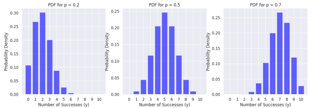
The likelihood function often involves products of probabilities, which can be difficult to compute, especially with large datasets. To simplify the mathematics and mitigate numerical issues (such as underflow), we often take the logarithm of the likelihood function, which transforms the product of probabilities into a sum. This is called the log-likelihood. Since logarithms are monotonic, maximizing the log-likelihood yields the same estimate as maximizing the likelihood.
Let’s return to the binomial distribution example, where we observe 7 heads out of 10 flips. The likelihood function is: L(p | y = 7, n = 10) = (10! / (7! * 3!)) * p^7 * (1 - p)^3 The log-likelihood function is: log L(p | y = 7, n = 10) = constant + 7 * log(p) + 3 * log(1 - p)
To find the MLE, we take the derivative of the log-likelihood with respect to p, set it equal to zero, and solve for p: d(log L) / dp = 7 / p - 3 / (1 - p) = 0 Solving this gives the MLE: p_MLE = 7 / 10 = 0.7 This means that the value of p that makes the observed data (7 heads in 10 flips) most likely is 0.7.
The most straightforward method to maximize the likelihood function is through calculus.
- Formulate the Likelihood Function: Write down the likelihood function based on the assumed probability distribution.
- Take the Logarithm: Convert the likelihood function to the log-likelihood function for computational convenience.
- Differentiate: Calculate the derivative of the log-likelihood function with respect to the parameters.
- Find Critical Points: Set the derivatives equal to zero and solve for the parameters. These are the potential maximum or minimum points.
- Check Second Derivative: To ensure the found point is a maximum, verify that the second derivative is negative.
For many real-world models, especially in machine learning, the likelihood function is too complicated to solve analytically. This is typical in deep learning or models with many parameters, where manually solving for the maximum by differentiating the likelihood function is not feasible. In some cases, the log-likelihood function might be non-convex, meaning it has multiple local maxima and minima, making analytical solutions even more difficult to obtain. Gradient descent can be used to navigate the landscape of the function and iteratively find an optimal point. Gradient descent allows us to compute the gradient of the log-likelihood with respect to the parameters and iteratively adjust the parameters to maximize the likelihood. Gradient descent is explained here.
Once the parameters are estimated, they are used to make predictions on new, unseen data. For instance, in a logistic regression model, the estimated coefficients are used to compute the probability of the binary outcomes for new data points. The estimated parameters are tested on validation datasets to ensure that the model generalizes well. This helps in understanding how well the model performs on new, unseen data and ensures that the MLE does not overfit the training data.
- Cross-entropy loss is used in classification tasks where the output of a model represents the probability distribution over classes. In logistic regression or neural networks with softmax activation, cross-entropy loss is derived from MLE. We assume that the labels follow a categorical distribution, and MLE attempts to maximize the likelihood of observing the correct label given the predicted probabilities. Minimizing the negative log-likelihood is the same as minimizing the cross-entropy loss.
- MSE is commonly used in regression tasks where the model predicts a continuous output. When using linear regression, if we assume that the errors (residuals) between the predicted values and true values follow a normal distribution, then MLE of the model parameters corresponds to minimizing the MSE. The normal distribution assumption leads to the least squares objective as the best estimate of the parameters.
But how does MLE compares with the four properties of estimators we talked about?
- In General MLEs are not guaranteed to be unbiased, especially in small sample sizes. For example, in estimating the variance of a normal distribution, the MLE is biased unless a correction factor is applied (the sample variance formula divides by n−1 instead of n). MLEs tend to become asymptotically unbiased, meaning that as the sample size grows large, the bias diminishes and E[θ^] converges to the true parameter θ.
- MLEs are generally consistent under regularity conditions, meaning that with a sufficiently large sample size, the MLE will converge to the true parameter value. The assumptions for consistency include that the model is correctly specified and that the likelihood function satisfies certain smoothness and regularity conditions. As more data becomes available, the likelihood function becomes more peaked around the true parameter value, allowing the MLE to “lock in” on the true parameter.
- MLEs are asymptotically efficient, meaning that for large sample sizes, they achieve the minimum variance among all consistent estimators. The variance of the MLE approaches the CRLB in large samples, making MLE highly desirable in practice for large datasets. For small sample sizes, MLE may not always be efficient. In certain cases, there may be other estimators that have smaller variances. Cramér-Rao Lower Bound (CRLB) gives the minimum variance that any unbiased estimator can achieve. If an estimator reaches this bound, it’s considered efficient, meaning it has the lowest possible variance among all unbiased estimators.
- MLE is often based on sufficient statistics. For example, in the case of the normal distribution, the sample mean and variance are sufficient statistics for estimating the parameters μ and σ2. By maximizing the likelihood function, MLE naturally incorporates all relevant information from the sufficient statistic. If a sufficient statistic exists for a model, MLE will typically make use of it to estimate the parameters.
- Under regularity conditions, the distribution of the MLE approaches a normal distribution centered around the true parameter value with a variance that depends on the Fisher Information. This property makes MLE particularly useful for constructing confidence intervals and hypothesis tests in large samples. Higher Fisher information implies a more concentrated distribution and thus a more precise estimate.
For more mathematical rigor I would recommend reading this paper (though totally optional). MLE is prominent in many parametric models like logistic regression, naive Bayes, and Gaussian Mixture Models. Other methods (Bayesian inference, least squares, hinge loss, decision trees, etc.) optimize different criteria or operate under different assumptions (e.g., maximum margin, reward maximization, impurity reduction) rather than focusing on likelihood maximization. MLE is just one method but most popular one!
Bayesian methods use probability distributions to model uncertainty about parameters. Instead of estimating a single value for a parameter, Bayesian methods estimate a posterior distribution by combining the likelihood (which may come from MLE) with a prior distribution on the parameters. We will talk about this method in another tutorial as bayesian methods can be computationally expensive in practice.
Thanks for reading. I hope this helped you get an idea how things work behind the scene in machine learning using mathematics. I will keep adding more topics here or maybe in another tutorial as this one is getting longer! If you are interested in joining our course, feel free to get started today. Also, don’t forget to grab these notes:
-
Sale Product on sale
 Linear Algebra For Machine Learning And Data Science
40.00$Original price was: 40.00$.24.99$Current price is: 24.99$. -
Sale Product on sale
 Probability and Statistics for Machine Learning and Data Science
30.00$Original price was: 30.00$.19.00$Current price is: 19.00$.
Sources And Additional Resources:
- Dennis Davis YouTube Channel
- Introductory Statistics By BARBARA ILLOWSKY and SUSAN DEAN
- Introduction to Probability Dimitri P. Bertsekas and John N. Tsitsiklis
- Introduction to Mathematical Statistics by Robert V. Hogg
- A mathematical theory of communication
- http://www.stat.columbia.edu/~liam/teaching/4107-fall05/notes3.pdf
- Tutorial on maximum likelihood estimation by Jae Myung
- https://www.stat.rice.edu/~dobelman/courses/texts/qualify/MLE.survey.Norden.Both.IMS.1972.pdf
- https://www.mit.edu/~rplevy/pmsl_textbook/chapters/pmsl_4.pdf
Amritesh Kumar
I believe you are not dumb or unintelligent; you just never had someone who could simplify the concepts you struggled to understand. My goal here is to simplify AI for all. Please help me improve this platform by contributing your knowledge on machine learning and data science, or help me improve current tutorials. I want to keep all the resources free except for support and certifications. Email me @amriteshkr18@gmail.com.

